Fitting parameters in a ModelingToolkit model

The following example demonstrates how to fit the parameters in a ModelingToolkit model using the function ControlSystemIdentification.nonlinear_pem. The nonlinear prediction-error method (PEM) uses a state estimator (Unscented Kalman Filter) underneath the hood to estimate the state of the system given the available measurements. This offers a very robust way of fitting parameters of a dynamical system, even when the model is imperfect and we cannot measure the entire state vector. This example is a continuation of the quadruple-tank example from Example: Quad tank.

The steps taken in this example are:

1. Define the ModelingToolkit model.
2. Obtain functions for the dynamics and the output of the system.
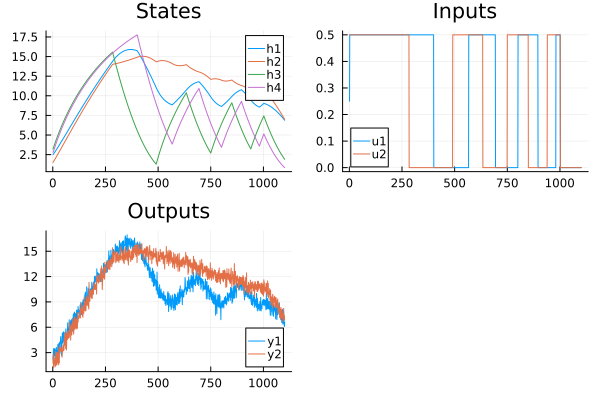
3. Generate some data to use for the estimation.
4. Specify properties of the prediction-error method and estimate the parameters using ControlSystemIdentification.nonlinear_pem.

Define the model

When we define the MTK model, we give defaults for all parameters:

using ControlSystemIdentification, ModelingToolkit, LeastSquaresOptim, SeeToDee, LowLevelParticleFilters, LinearAlgebra, Random, Plots # Load the
using ModelingToolkit: D_nounits as D
t = ModelingToolkit.t_nounits
ssqrt(x) = √(max(x, zero(x)) + 1e-3) # For numerical robustness at x = 0
@register_symbolic ssqrt(x)

@mtkmodel QuadtankModel begin
    @parameters begin
        k1 = 1.4
        k2 = 1.4
        g = 9.81
        A = 5.1
        a = 0.03
        γ = 0.25
    end
    begin
        A1 = A2 = A3 = A4 = A
        a1 = a3 = a2 = a4 = a
        γ1 = γ2 = γ
    end
    @variables begin
        h(t)[1:4] = 0
        u(t)[1:2] = 0
    end
    @equations begin
        D(h[1]) ~ -a1/A1 * ssqrt(2g*h[1]) + a3/A1*ssqrt(2g*h[3]) +     γ1*k1/A1 * u[1]
        D(h[2]) ~ -a2/A2 * ssqrt(2g*h[2]) + a4/A2*ssqrt(2g*h[4]) +     γ2*k2/A2 * u[2]
        D(h[3]) ~ -a3/A3*ssqrt(2g*h[3])                          + (1-γ2)*k2/A3 * u[2]
        D(h[4]) ~ -a4/A4*ssqrt(2g*h[4])                          + (1-γ1)*k1/A4 * u[1]
    end
end

@named mtkmodel = QuadtankModel()

\[\begin{align} \frac{\mathrm{d} h\left( t \right)_{1}}{\mathrm{d}t} &= \frac{a ssqrt\left( 2 g h\left( t \right)_{3} \right)}{A} + \frac{\mathtt{k1} u\left( t \right)_{1} \gamma}{A} + \frac{ - a ssqrt\left( 2 g h\left( t \right)_{1} \right)}{A} \\ \frac{\mathrm{d} h\left( t \right)_{2}}{\mathrm{d}t} &= \frac{\mathtt{k2} u\left( t \right)_{2} \gamma}{A} + \frac{ - a ssqrt\left( 2 g h\left( t \right)_{2} \right)}{A} + \frac{a ssqrt\left( 2 g h\left( t \right)_{4} \right)}{A} \\ \frac{\mathrm{d} h\left( t \right)_{3}}{\mathrm{d}t} &= \frac{\mathtt{k2} u\left( t \right)_{2} \left( 1 - \gamma \right)}{A} + \frac{ - a ssqrt\left( 2 g h\left( t \right)_{3} \right)}{A} \\ \frac{\mathrm{d} h\left( t \right)_{4}}{\mathrm{d}t} &= \frac{\mathtt{k1} u\left( t \right)_{1} \left( 1 - \gamma \right)}{A} + \frac{ - a ssqrt\left( 2 g h\left( t \right)_{4} \right)}{A} \end{align}\]

Obtain dynamics functions

We then specify the inputs and outputs of this model, since they are arrays in this example, we call collect to turn them into scalars. To obtain a dynamics function on the form

\[\dot x = f(x, u, p, t)\]

from MTK, we call ModelingToolkit.generate_control_function. This example assumes that the system model has an external input, $u$. If your example does not have this, you may leave this argument empty. This returns two versions of this function, where the second one operates in place (modifying its first argument). This function also returns the state variables chosen, the parameters of the model as well as a simplified system with inputs and outputs. The function returned from ModelingToolkit.generate_control_function expects all the parameters of the system to be provided, but we only want to optimize a few of them. We thus wrap this function in discrete_dynamics_mtk in order to insert the optimized parameters into a parameter array that contains also the non-optimized parameters. We make use of the function similar to ensure that the final parameter array has the correct type (Dual numbers for AD will be used).

For good performance, we wrap all the glue code in a function get_mtk_dynamics so that we avoid the use of too many global variables.

mtkmodel = complete(mtkmodel)
inputs = [collect(mtkmodel.u);]
outputs = [collect(mtkmodel.h[1:2]);]
tunable_p = [mtkmodel.k1, mtkmodel.k2, mtkmodel.A, mtkmodel.γ] # Provided in the same order as p_guess

function get_mtk_dynamics(mtkmodel, inputs, outputs, tunable_p) # A wrapper function to avoid using global variables

    (f_oop, f_ip), statevars, p, io_sys = ModelingToolkit.generate_control_function(mtkmodel, inputs; outputs, split=false)

    continuous_dynamics = f_oop # This is ẋ = f(x, u, p, t)
    inner_discrete_dynamics = SeeToDee.Rk4(continuous_dynamics, Ts::Float64) # x⁺ = f(x, u, p, t)
    tunable_indices = [findfirst(isequal(pi), p) for pi in tunable_p] # Figure out what indices of the parameter array correspond to our tunable parameters
    p0 = [ModelingToolkit.defaults(io_sys)[pi] for pi in p]
    full_p = deepcopy(p0)
    output_indices = [findfirst(isequal(yi), statevars) for yi in outputs] # Figure out what indices of the state array correspond to our outputs

    function discrete_dynamics_wrapper(x, u, p, t)
        opt_p = similar(p, length(full_p)) # Create an array of correct length and element type to host the full parameter vector
        opt_p .= full_p # Write all the initial parameters into this new array
        opt_p[tunable_indices] .= p # Overwrite the tunable parameters with the optimization variable
        inner_discrete_dynamics(x, u, opt_p, t) # Call the discretized dynamics function from MTK
    end

    mtk_measurement(x,u,p,t) = x[output_indices]

    discrete_dynamics_wrapper, mtk_measurement
end

Ts = 1.0    # Sample interval used for discretization
discrete_dynamics, measurement = get_mtk_dynamics(mtkmodel, inputs, outputs, tunable_p)

Simulate measurement data

We generate some data to use for the estimation by simulating the system

ny = 2      # Dimension of measurements
nu = 2      # Dimension of inputs
p_true = [1.6, 1.6, 4.9, 0.2] # True parameters

Random.seed!(1)
# Generate input signal
Tperiod = 200
tvec = 0:Ts:1000
u1 = vcat.(0.25 .* sign.(sin.(2pi/Tperiod .* (tvec ./ 40).^2)) .+ 0.25)
u2 = vcat.(0.25 .* sign.(sin.(2pi/Tperiod .* (tvec ./ 40).^2 .+ pi/2)) .+ 0.25)
u  = vcat.(u1,u2)
u = [u; 0 .* u[1:100]]
x0 = [2.5, 1.5, 3.2, 2.8] # Initial state
x = LowLevelParticleFilters.rollout(discrete_dynamics, x0, u, p_true; Ts)[1:end-1] # Simulate
y = measurement.(x, u, 0, 0) # Generate measured outputs
y = [y .+ 0.5randn(ny) for y in y] # Add some measurement noise
Y = reduce(hcat, y) # Go from vector of vectors to a matrix
U = reduce(hcat, u) # Go from vector of vectors to a matrix
plot(
    plot(reduce(hcat, x)', title="States", lab=["h1" "h2" "h3" "h4"]),
    plot(U', title="Inputs", lab=["u1" "u2"]),
    plot(Y', title="Outputs", lab=["y1" "y2"]),
)

Perform estimation

We package the input and output data arrays Y and U into an iddata object and define some initial guesses for the parameters and the initial state. We also define the covariance matrices for the process and measurement noise. These matrices allow us to specify how much we "trust" the model and how much we trust the measurements. We finally call ControlSystemIdentification.nonlinear_pem to estimate the parameters.

d = iddata(Y, U, Ts)
x0_guess = [2.5, 1.5, 1, 2]     # Guess for the initial condition (initial state)
p_guess  = [1.4, 1.4, 5.1, 0.25] # Initial guess for the parameters

R1 = Diagonal([0.1, 0.1, 0.1, 0.1]) # This controls how much we trust the model (covariance of the process noise)
R2 = 100*Diagonal(0.5^2 * ones(ny)) # This controls how much we trust the measurements (covariance of the measurement noise)

model = ControlSystemIdentification.nonlinear_pem(d, discrete_dynamics, measurement, p_guess, x0_guess, R1, R2, nu)

NonlinearPredictionErrorModel
  p: [1.6130151977611773, 1.5995448472434575, 4.887899044534598, 0.20437506116084214]
  x0: [2.5590156863624642, 1.674133802252665, 2.890730509103397, 2.114949939609547]
  Ts: 1.0
  ny = 2, nu = 2, nx = 4

The estimated parameters are now available as model.p and they should be close to the true values p_true = [1.6, 1.6, 4.9, 0.2].

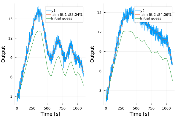
We may visualize how well the model performs by simulating it and comparing the results to the measured data:

simplot(model, d, layout=2)

The fitting should be quite fast:

using BenchmarkTools
@btime ControlSystemIdentification.nonlinear_pem(d, discrete_dynamics, measurement, p_guess, x0_guess, R1, R2, nu)

101.731 ms (873689 allocations: 97.10 MiB)