Fault detection

This is also a video tutorial, available below:

Fault detection using state estimation

This tutorial explores the use of a Kalman filter for fault detection in a thermal system

Modeling
Filtering
Maximum-likelihood estimation of covariance and model parameters
Monitor prediction-error Z-score to detect faults
- A fault may be faulty sensor or unexpected temperature fluctuations

using DelimitedFiles, Plots, Dates
using LowLevelParticleFilters, LinearAlgebra, StaticArrays
using Optim
using ADTypes: AutoForwardDiff

Look at the data

plot(time, y, ylabel="Temperature", legend=false)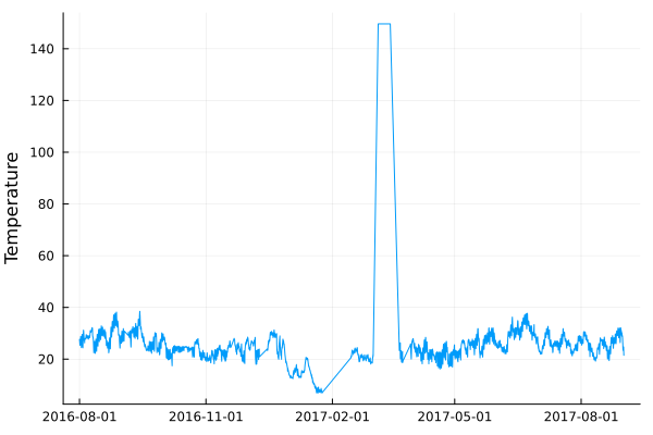

timev = Dates.value.(time)  ./ 1000 # A numerical time vector, time was in milliseconds
plot(diff(timev), yscale=:log10, title="Time interval between measurement points", legend=false)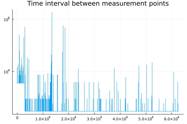

Samples are not evenly spaced (lots of missing data), but the interval is always a multiple of the smallest interval, which we take as the sample interval Ts

intervals = sort(unique(diff(timev)))
intervals ./ intervals[1]
Ts = intervals[1]

Tf = intervals[end] - intervals[1]

We expand the data arrays such that we can treat them as having a constant sample interval, time points where there is no data available are indicated as missing. Each measurement is a vector of length one, and a vector of which all entries are missing is treated as a missing measurement by the filters in this package, see Missing data and outliers.

time_full = range(timev[1], timev[end], step=Ts)

available_inds = [findfirst(==(t), time_full) for t in timev]

y_full = fill(NaN, length(time_full))
y_full[available_inds] .= y
y_full = replace(y_full, NaN=>missing)
y_full = SVector{1}.(y_full)

Design Kalman filter

Modeling

A simple model of temperature change is

\[\dot T(t) = \alpha \big(T(t) - T_{env}(t)\big) + w(t)\]

Where $T$ is the temperature of the system, $T_{env}$ the temperature of the environment and $w$ represents thermal energy added or removed by unmodeled sources.

Since we have no knowledge of $T_{env}$ and $w$, but we observe that they vary slowly, we add yet another state variable to the model corresponding to an integrating disturbance model:

\[\begin{aligned} \dot T(t) &= z(t) + b_T w_T(t) \\ \dot z(t) &= b_z w_z(t) \end{aligned}\]

This model is linear, and can be written on the form

\[\begin{aligned} \dot x &= Ax + Bw \\ y &= Cx + e \end{aligned}\]

with $A$ matrix

\[A = \begin{bmatrix} 0 & 1 \\ 0 & 0 \end{bmatrix}\]

which, when discretized (assuming unit sample interval), becomes

\[A = \begin{bmatrix} 1 & 1 \\ 0 & 1 \end{bmatrix}\]

A,B,C,D = SA[1.0 1; 0 1], @SMatrix(zeros(2,0)), SA[1.0 0], 0;

Picking covariance matrices

R1 = 1e-4LowLevelParticleFilters.double_integrator_covariance(1) |> SMatrix{2,2}
R2 = SA[0.1^2;;]
d0 = LowLevelParticleFilters.SimpleMvNormal(SA[y[1], 0], SA[100.0 0; 0 0.1])
kf = KalmanFilter(A,B,C,D,R1,R2,d0; Ts)

KalmanFilter{StaticArraysCore.SMatrix{2, 2, Float64, 4}, StaticArraysCore.SMatrix{2, 0, Float64, 0}, StaticArraysCore.SMatrix{1, 2, Float64, 2}, Matrix{Float64}, StaticArraysCore.SMatrix{2, 2, Float64, 4}, StaticArraysCore.SMatrix{1, 1, Float64, 1}, LowLevelParticleFilters.SimpleMvNormal{StaticArraysCore.SVector{2, Float64}, StaticArraysCore.SMatrix{2, 2, Float64, 4}}, StaticArraysCore.SVector{2, Float64}, StaticArraysCore.SMatrix{2, 2, Float64, 4}, Float64, LowLevelParticleFilters.NullParameters, Float64}([1.0 1.0; 0.0 1.0], 2×0 StaticArraysCore.SMatrix{2, 0, Float64, 0} with indices SOneTo(2)×SOneTo(0), [1.0 0.0], Matrix{Float64}(undef, 1, 0), [2.5e-5 5.0e-5; 5.0e-5 0.0001], [0.010000000000000002;;], LowLevelParticleFilters.SimpleMvNormal{StaticArraysCore.SVector{2, Float64}, StaticArraysCore.SMatrix{2, 2, Float64, 4}}([27.63677025, 0.0], [100.0 0.0; 0.0 0.1]), [27.63677025, 0.0], [100.0 0.0; 0.0 0.1], 0, 300.0, LowLevelParticleFilters.NullParameters(), 1.0, 2, 0, 1, SignalNames(["x1", "x2"], String[], ["y1"], "KF"))

Perform filtering

When data is missing, the call to correct! is omitted, while the prediction step is still performed. forward_trajectory does this automatically for the time steps where the measurement is missing.

u_full = [@SVector(zeros(0)) for y in y_full];

start = 1 # Change this value to display different parts of the data set
N = 1000  # Number of data points to include (to limit plot size in the docs, plot with Plots.plotly() and N = length(y_full) to see the full data set with the ability to zoom interactively in the plot)
inds = (1:N) .+ (start-1)

sol = forward_trajectory(kf, u_full[inds], y_full[inds])

sol.ll

-33.701475549446464

The Z-score of the prediction error, $\sqrt{e^T S^{-1} e}$, where $S$ is the covariance of the prediction error $e$, can be computed from the quantities stored in the solution object. sol.S contains the Cholesky factorization of $S$, and sol.S[k] is missing for time steps where the measurement is missing, for which we return NaN.

zscores(sol) = [S === missing ? NaN : sqrt(e'*(S\e)) for (e, S) in zip(sol.e, sol.S)]
σs = zscores(sol)

Smoothing

For good measure, we also perform smoothing, computing

\[x(k \,|\, T_f)\]

as opposed to filtering which is computing

\[x(k \,|\, k)\]

or prediction

\[x(k \,|\, k-1)\]

smoothsol = smooth(sol)

Visualize the filtered and smoothed trajectories

timevec = range(0, step=Ts, length=length(sol.y))

plot(smoothsol,
    plotx   = false, # prediction
    plotxt  = true,  # filtered
    plotxT  = true,  # smoothed
    plotRt  = true,
    plotRT  = true,
    plotyh  = false,
    plotyht = true,
    size = (650,600), seriestype = [:line :line :scatter :line], link = :x,
)
plot!(timevec, reduce(hcat, smoothsol.xT)[1,:], sp=3, label="Smoothed")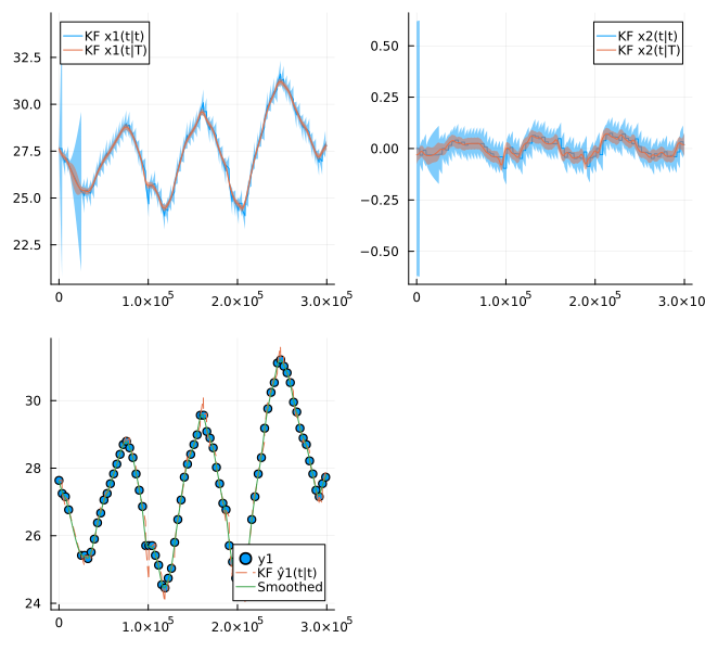

Estimate the dynamics covariance using maximum-likelihood estimation (MLE)

Since we have a single parameter only, we may plot the loss landscape.

svec = exp10.(range(-5, -2, length=30)) # Covariance values to try

# Compute the log-likelihood for all covariance values
lls = map(svec) do s
	R1 = s*LowLevelParticleFilters.double_integrator_covariance(1) |> SMatrix{2,2}
	kf = KalmanFilter(A,B,C,D,R1,R2,d0; Ts)
	loglik(kf, u_full, y_full)
end

plot(svec, lls, xscale=:log10, title="Log-likelihood estimation")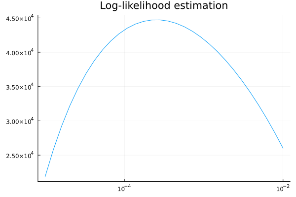

Get the covariance parameter associated with the maximum likelihood:

svec[argmax(lls)]

0.0002807216203941176

Optimize "friction" and covariance jointly

We can add some damping to the velocity state variable in the double-integrator model. When doing so, we should also estimate the full covariance matrix of the dynamics noise. This gives us an estimation problem with 1 + 3 parameters, 3 for the upper triangle of the Cholesky factor of the covariance matrix. We use the log-Cholesky parameterization LowLevelParticleFilters.cov_from_logchol, in which the diagonal entries of the Cholesky factor are the exponentials of the corresponding parameters, while the off-diagonal entries are equal to the parameters. This parameterization maps every parameter vector to a valid, symmetric and positive-definite covariance matrix, and correlations of both signs are representable.

A double integrator has the dynamics matrix

\[\begin{bmatrix} 1 & 1 \\ 0 & 1 \end{bmatrix}\]

By modifying this to

\[\begin{bmatrix} 1 & 1 \\ 0 & \alpha \end{bmatrix}\]

where $0 < \alpha < 1$, we can add some damping to the velocity, i.e., if no force is acting on it it will eventually slow down to velocity zero. It's not quite correct to call the parameter $\alpha$ a "damping term", the formulation $\beta = 1 - \alpha$ would be closer to an actual discrete-time damping factor. To ensure that $\alpha$ remains in the interval $(0, 1)$, we optimize a parameter $\theta_\alpha$ and let $\alpha = 1/(1 + e^{-\theta_\alpha})$.

The covariance matrix used above, double_integrator_covariance, has rank one and can thus not be represented by the log-Cholesky parameterization. As initial guess, we instead use the full-rank covariance matrix double_integrator_covariance_smooth, which corresponds to continuous-time white noise acting on the velocity, scaled by the maximum-likelihood estimate of the scale parameter found above.

R1_init = svec[argmax(lls)]*LowLevelParticleFilters.double_integrator_covariance_smooth(1) |> SMatrix{2,2}
logistic(x) = 1/(1 + exp(-x))
logit(α) = log(α/(1 - α))
α_init = 0.99

params = [LowLevelParticleFilters.logchol_from_cov(R1_init); logit(α_init)]

function get_opt_kf(θ)
	T = eltype(θ)
	R1 = LowLevelParticleFilters.cov_from_logchol(θ[1:3], Val(2))
	α = logistic(θ[4])
	A = SA[1 1; 0 α]
	d0T = LowLevelParticleFilters.SimpleMvNormal(T.(d0.μ), T.(d0.Σ))
	KalmanFilter(A,B,C,D,R1,R2,d0T; Ts, check=false)
end

cost(θ) = -loglik(get_opt_kf(θ), u_full, y_full)

cost(params)

-45186.17684037944

The element type of the initial state distribution is converted to the element type of the parameter vector, which is required when the gradient is computed using ForwardDiff.

Optimize

res = Optim.optimize(
    cost,
    params,
    LBFGS(),
    Optim.Options(
        show_trace        = true,
        show_every        = 5,
        iterations        = 1000,
		x_abstol 	      = 1e-7,
    ),
	autodiff = AutoForwardDiff(),
)
get_opt_kf(res.minimizer).R1

2×2 StaticArraysCore.SMatrix{2, 2, Float64, 4} with indices SOneTo(2)×SOneTo(2):
 0.000104159  0.000198335
 0.000198335  0.000377662

The initial guess was

R1_init

2×2 StaticArraysCore.SMatrix{2, 2, Float64, 4} with indices SOneTo(2)×SOneTo(2):
 9.35739e-5   0.000140361
 0.000140361  0.000280722

The optimized parameter $\alpha$ and the log-likelihood before and after the optimization are

logistic(res.minimizer[4]), -cost(params), -res.minimum

(0.904142590285098, 45186.17684037944, 46645.93419507695)

Visualize optimized filtering trajectory

kf2 = get_opt_kf(res.minimizer)
sol2 = forward_trajectory(kf2, u_full[inds], y_full[inds])
σs2 = zscores(sol2)

smoothsol2 = smooth(sol2)

plot(smoothsol2, plotx=false, plotxt=true, plotRt=true, plotyh=false, plotyht=true, size=(650,600), seriestype=[:line :line :scatter :line], link=:x)
plot!(timevec, reduce(hcat, smoothsol2.xT)[1,:], sp=3, label="Smoothed")

outliers = findall(σs2 .> 5)
vline!([timevec[outliers]], sp=3, label=false)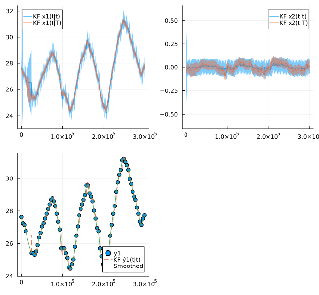

Fault detection

We implement a simple fault detector using Z-scores. When the Z-score is higher than 4, we consider it a fault. The Z-score is NaN for time steps where the measurement is missing, these time steps are not drawn in the plot.

scatter(timevec, σs2, ms=2, label="Z-score"); hline!([1 2 3 4], label=false)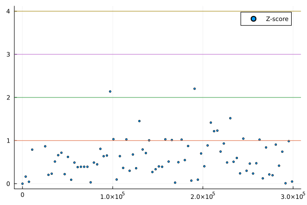

(change the value of the variable start to see different parts of the data set, e.g., set start = 30_000)

Z-scores may not capture large outliers if they occur when the estimator is very uncertain Does Z-score correlate with "velocity", i.e., are faults correlated with large continuous slopes in the data?

sol_full = forward_trajectory(kf2, u_full, y_full)
σs_full = zscores(sol_full)
scatter(abs.(getindex.(sol_full.xt, 2)), σs_full, ylabel="Z-score", xlabel="velocity")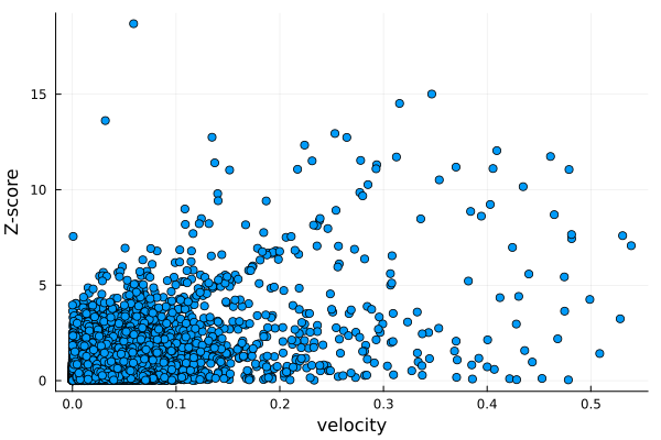

not really, it looks like large Z-scores can appear even when the estimated velocity is small.

Alternative fault-detection strategies

In this tutorial, we used the Z-score of the prediction error to detect faults. A Kalman filter, being a statistical estimator, maintains a belief about the state of the system, whenever this belief is inconsistent with fault-free operation, we may experiencing a fault. Below are some alternative ways in which we can detect faults using a Kalman filter:

A single measurement has a Z-score larger than a threshold. The benefit of this approach is that it can isolate issues to a single sensor.
The entire measurement vector has a large Z-score. This can detect issues that cause unexpected correlation in the output, but where each individual output looks as expected on its own.
The filter may be augmented with a disturbance model. If the estimated disturbance is larger than expected, e.g., significantly different from zero, it may indicate a fault. See How to tune a Kalman filter and Disturbance gallery for more information on how to do this.
Parameters of the system may be modeled as time-varying and estimated online. If, e.g., an estimated gain parameter decreases significantly, it may indicate a fault. This is similar in spirit to adding a disturbance model, but instead of estimating an input disturbance, we estimate a property of the system. See Joint state and parameter estimation for an example of this.
An article suggesting several consistency checks similar to the Z-score check used here is "New Kalman filter and smoother consistency tests" by Gibbs, all of which can be readily computed from the quantities saved in the KalmanFilteringSolution object and the result of smooth. One suggestion is to use the filter error and associated filter-error covariance instead of the prediction error, another one is similar but using a smoothed error instead. The last suggestion is to use the smoothed stat error in a similar check.

Summary

A state estimator can indicate faults when the error is larger than expected
What is expected is determined by the model

The notebook used in the tutorial is available here:

identification_12_fault_detection.jl on GitHub