Validation

A number of functions are made available to assist in validation of the estimated models. We illustrate by an example

Generate some test data:

using ControlSystemIdentification, ControlSystemsBase, Random
using ControlSystemIdentification: newpem
Random.seed!(1)
T          = 200
nx         = 2
nu         = 1
ny         = 1
x0         = randn(nx)
σy         = 0.5
sim(sys,u) = lsim(sys, u, 1:T)[1]
sys        = tf(1, [1, 2*0.1, 0.1])
sysn       = tf(σy, [1, 2*0.1, 0.3])
# Training data
u          = randn(nu,T)
y          = sim(sys, u)
yn         = y + sim(sysn, randn(size(u)))
dn         = iddata(yn, u, 1)
# Validation data
uv         = randn(nu, T)
yv         = sim(sys, uv)
ynv        = yv + sim(sysn, randn(size(uv)))
dv         = iddata(yv, uv, 1)
dnv        = iddata(ynv, uv, 1)

InputOutput data of length 200, 1 outputs, 1 inputs, Ts = 1

We then fit a couple of models

res = [newpem(dn, nx, focus=:prediction) for nx = [2,3,4]];

Iter     Function value   Gradient norm
     0     8.214820e+01     4.786930e+02
 * time: 4.601478576660156e-5
    50     1.367893e+01     1.347632e+02
 * time: 0.021926164627075195
   100     1.098123e+01     2.451721e-01
 * time: 0.032731056213378906
Iter     Function value   Gradient norm
     0     6.941423e+01     6.057682e+02
 * time: 3.981590270996094e-5
    50     1.905270e+01     8.542130e+02
 * time: 0.04700803756713867
Iter     Function value   Gradient norm
     0     5.781936e+01     6.010229e+02
 * time: 4.1961669921875e-5
    50     7.805465e+00     4.607879e+01
 * time: 0.04195713996887207

After fitting the models, we validate the results using the validation data and the functions simplot and predplot (cf. Matlab sys.id's compare):

using Plots
ω   = exp10.(range(-2, stop=log10(pi), length=150))
fig = plot(layout=4, size=(1000,600))
for i in eachindex(res)
    sysh, x0h, opt = res[i]
    simplot!( sysh, dnv, x0h; sp=1, ploty=false)
    predplot!(sysh, dnv, x0h; sp=2, ploty=false)
end
plot!(dnv.y' .* [1 1], lab="y", l=(:dash, :black), sp=[1 2])
bodeplot!((getindex.(res,1)),                     ω, link = :none, balance=false, plotphase=false, subplot=3, title="Process", linewidth=2*[4 3 2 1])
bodeplot!(innovation_form.(getindex.(res,1)),     ω, link = :none, balance=false, plotphase=false, subplot=4, linewidth=2*[4 3 2 1])
bodeplot!(sys,                                    ω, link = :none, balance=false, plotphase=false, subplot=3, lab="True", l=(:black, :dash), legend = :bottomleft, title="System model")
bodeplot!(innovation_form(ss(sys),syse=ss(sysn)), ω, link = :none, balance=false, plotphase=false, subplot=4, lab="True", l=(:black, :dash), ylims=(0.1, 100), legend = :bottomleft, title="Noise model")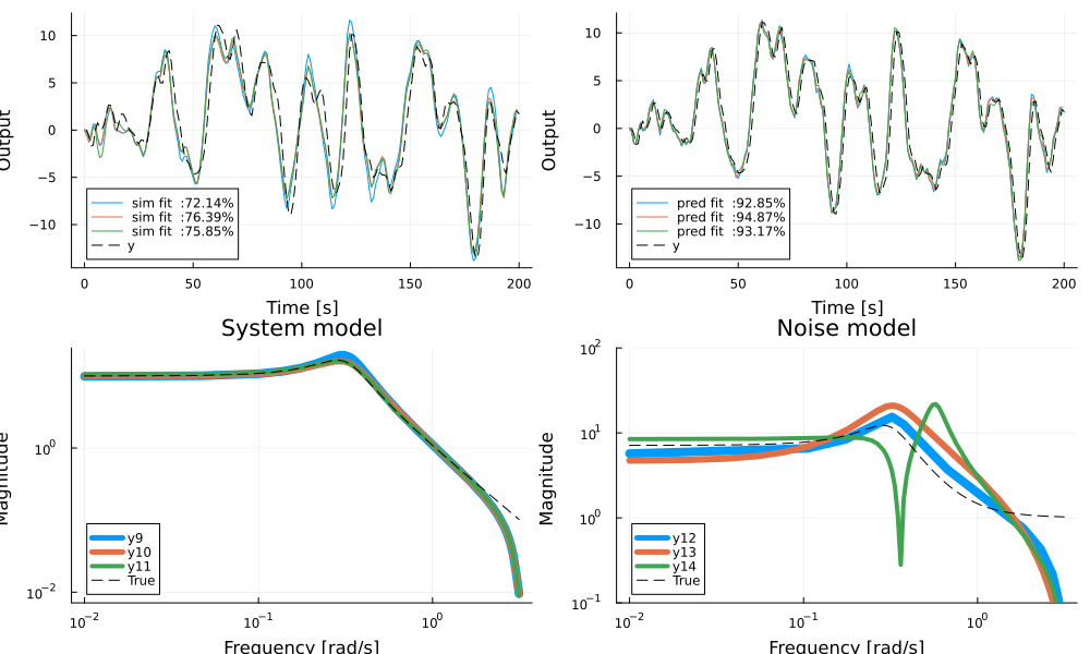

In the figure, simulation output is compared to the true model on the top left and prediction on top right. The system models and noise models are visualized in the bottom plots. All models capture the system dynamics reasonably well, but struggle slightly with capturing the gain of the noise dynamics. The true system has 4 poles (two in the process and two in the noise process) but a simpler model may sometimes work better.

Prediction models may also be evaluated using a h-step prediction, here h is short for "horizon".

figh = plot()
for i in eachindex(res)
    sysh, x0h, opt = res[i]
    predplot!(sysh, dnv, x0h, ploty=false, h=5)
end
plot!(dnv.y', lab="y", l=(:dash, :black))
figh

It's generally a good idea to validate estimated model with a prediction horizon larger than one, in particular, it may be valuable to verify the performance for a prediction horizon that corresponds roughly to the dominant time constant of the process.

Different length predictors

When the prediction horizon gets longer, the mapping from $u \rightarrow ŷ$ approaches that of the simulation system, while the mapping $y \rightarrow ŷ$ gets smaller and smaller.

using LinearAlgebra
G   = c2d(DemoSystems.resonant(), 0.1)
K   = kalman(G, I(G.nx), I(G.ny))
sys = add_input(G, K, I(G.ny)) # Form an innovation model with inputs u and e

T = 10000
u = randn(G.nu, T)
e = 0.1randn(G.ny, T)
y = lsim(sys, [u; e]).y
d = iddata(y, u, G.Ts)
Gh,_ = newpem(d, G.nx, zeroD=true)

# Create predictors with different horizons
p1   = observer_predictor(Gh)
p2   = observer_predictor(Gh, h=2)
p10  = observer_predictor(Gh, h=10)
p100 = observer_predictor(Gh, h=100)

bodeplot([p1, p2, p10, p100], plotphase=false, lab=["1" "" "2" "" "10" "" "100" ""])
bodeplot!(sys, ticks=:default, plotphase=false, l=(:black, :dash), lab=["sim" ""], title=["From u" "From y"])

The prediction error as a function of prediction horizon approaches the simulation error.

using Statistics
hs = [1:40; 45:5:80]
perrs = map(hs) do h
    yh = predict(Gh, d; h)
    ControlSystemIdentification.rms(d.y - yh) |> mean
end
serr = ControlSystemIdentification.rms(d.y - simulate(Gh, d)) |> mean

plot(hs, perrs, lab="Prediction errors", xlabel="Horizon", ylabel="RMS error")
hline!([serr], lab="Simulation error", l=:dash, legend=:bottomright, ylims=(0, Inf))

Validation API

StatsAPI.predict — Function

predict(ARX::TransferFunction, d::InputOutputData)

One step ahead prediction for an ARX process. The length of the returned prediction is length(d) - max(na, nb)

Example:

julia> predict(tf(1, [1, -1], 1), iddata(1:10, 1:10))
9-element Vector{Int64}:
  2
  4
  6
  8
 10
 12
 14
 16
 18

source

predict(sys, d::AbstractIdData, args...)
predict(sys, y, u, x0 = nothing)

Video tutorials

Relevant video tutorials are available here: