LowLevelParticleFilters

This is a library for state estimation, that is, given measurements $y(t)$ from a dynamical system, estimate the state vector $x(t)$. Throughout, we assume dynamics on the form

\[\begin{aligned} x(t+1) &= f(x(t), u(t), p, t, w(t))\\ y(t) &= g(x(t), u(t), p, t, e(t)) \end{aligned}\]

or the linear version

\[\begin{aligned} x(t+1) &= Ax(t) + Bu(t) + w(t)\\ y(t) &= Cx(t) + Du(t) + e(t) \end{aligned}\]

where $x$ is the state vector, $u$ an input, $p$ some form of parameters, $t$ is the time and $w,e$ are disturbances (noise). Throughout the documentation, we often call the function $f$ dynamics and the function $g$ measurement.

The dynamics above describe a discrete-time system, i.e., the function $f$ takes the current state and produces the next state. This is in contrast to a continuous-time system, where $f$ takes the current state but produces the time derivative of the state. A continuous-time system can be discretized, described in detail in Discretization.

The parameters $p$ can be anything, or left out. You may write the dynamics functions such that they depend on $p$ and include parameters when you create a filter object. You may also override the parameters stored in the filter object when you call any function on the filter object. This behavior is modeled after the SciML ecosystem.

Depending on the nature of $f$ and $g$, the best method of estimating the state may vary. If $f,g$ are linear and the disturbances are additive and Gaussian, the KalmanFilter is an optimal state estimator. If any of the above assumptions fail to hold, we may need to resort to more advanced estimators. This package provides several filter types, outlined below.

Estimator types

We provide a number of filter types

• KalmanFilter. A standard Kalman filter. Is restricted to linear dynamics (possibly time varying) and Gaussian noise.
• SqKalmanFilter. A standard Kalman filter on square-root form (slightly slower but more numerically stable with ill-conditioned covariance).
• ExtendedKalmanFilter: For nonlinear systems, the EKF runs a regular Kalman filter on linearized dynamics. Uses ForwardDiff.jl for linearization. The noise model must be Gaussian.
• UnscentedKalmanFilter: The Unscented Kalman filter often performs slightly better than the Extended Kalman filter but may be slightly more computationally expensive. The UKF handles nonlinear dynamics and measurement model, but still requires an additive Gaussian noise model and assumes all posterior distributions are Gaussian, i.e., can not handle multi-modal posteriors.
• ParticleFilter: The particle filter is a nonlinear estimator. This version of the particle filter is simple to use and assumes that both dynamics noise and measurement noise are additive. Particle filters handle multi-modal posteriors.
• AdvancedParticleFilter: This filter gives you more flexibility, at the expense of having to define a few more functions. This filter does not require the noise to be additive and is thus the most flexible filter type.
• AuxiliaryParticleFilter: This filter is identical to ParticleFilter, but uses a slightly different proposal mechanism for new particles.
• DAEUnscentedKalmanFilter: An Unscented Kalman filter for differential-algebraic systems (DAE).

Functionality

This package provides

• Filtering, estimating $x(t)$ given measurements up to and including time $t$. We call the filtered estimate $x(t|t)$ (read as $x$ at $t$ given $t$).
• Smoothing, estimating $x(t)$ given data up to $T > t$, i.e., $x(t|T)$.
• Parameter estimation.

All filters work in two distinct steps.

1. The prediction step (predict!). During prediction, we use the dynamics model to form $x(t|t-1) = f(x(t-1), ...)$
2. The correction step (correct!). In this step, we adjust the predicted state $x(t|t-1)$ using the measurement $y(t)$ to form $x(t|t)$.

In general, all filters represent not only a point estimate of $x(t)$, but a representation of the complete posterior probability distribution over $x$ given all the data available up to time $t$. One major difference between different filter types is how they represent these probability distributions.

Particle filter

A particle filter represents the probability distribution over the state as a collection of samples, each sample is propagated through the dynamics function $f$ individually. When a measurement becomes available, the samples, called particles, are given a weight based on how likely the particle is given the measurement. Each particle can thus be seen as representing a hypothesis about the current state of the system. After a few time steps, most weights are inevitably going to be extremely small, a manifestation of the curse of dimensionality, and a resampling step is incorporated to refresh the particle distribution and focus the particles on areas of the state space with high posterior probability.

Defining a particle filter is straightforward, one must define the distribution of the noise df in the dynamics function, dynamics(x,u,p,t) and the noise distribution dg in the measurement function measurement(x,u,p,t). Both of these noise sources are assumed to be additive, but can have any distribution. The distribution of the initial state d0 must also be provided. An example for a linear Gaussian system is given below.

using LowLevelParticleFilters, LinearAlgebra, StaticArrays, Distributions, Plots

Define problem

n = 2   # Dimension of state
m = 1   # Dimension of input
p = 1   # Dimension of measurements
N = 500 # Number of particles

const dg = MvNormal(p,1.0)          # Measurement noise Distribution
const df = MvNormal(n,1.0)          # Dynamics noise Distribution
const d0 = MvNormal(randn(n),2.0)   # Initial state Distribution

Define linear state-space system (using StaticArrays for maximum performance)

const A = SA[0.97043   -0.097368
             0.09736    0.970437]
const B = SA[0.1; 0;;]
const C = SA[0 1.0]

Next, we define the dynamics and measurement equations, they both take the signature (x,u,p,t) = (state, input, parameters, time)

dynamics(x,u,p,t) = A*x .+ B*u
measurement(x,u,p,t) = C*x
vecvec_to_mat(x) = copy(reduce(hcat, x)') # Helper function

the parameter p can be anything, and is often optional. If p is not provided when performing operations on filters, any p stored in the filter objects (if supported) is used. The default if none is provided and none is stored in the filter is p = SciMLBase.NullParameters().

We are now ready to define and use a filter

pf = ParticleFilter(N, dynamics, measurement, df, dg, d0)

ParticleFilter{PFstate{StaticArraysCore.SVector{2, Float64}, Float64}, typeof(Main.dynamics), typeof(Main.measurement), Distributions.ZeroMeanIsoNormal{Tuple{Base.OneTo{Int64}}}, Distributions.ZeroMeanIsoNormal{Tuple{Base.OneTo{Int64}}}, Distributions.IsoNormal, DataType, Random.Xoshiro, SciMLBase.NullParameters}
  state: PFstate{StaticArraysCore.SVector{2, Float64}, Float64}
  dynamics: dynamics (function of type typeof(Main.dynamics))
  measurement: measurement (function of type typeof(Main.measurement))
  dynamics_density: Distributions.ZeroMeanIsoNormal{Tuple{Base.OneTo{Int64}}}
  measurement_density: Distributions.ZeroMeanIsoNormal{Tuple{Base.OneTo{Int64}}}
  initial_density: Distributions.IsoNormal
  resample_threshold: Float64 0.1
  resampling_strategy: LowLevelParticleFilters.ResampleSystematic <: LowLevelParticleFilters.ResamplingStrategy
  rng: Random.Xoshiro
  p: SciMLBase.NullParameters SciMLBase.NullParameters()
  threads: Bool false

With the filter in hand, we can simulate from its dynamics and query some properties

du = MvNormal(m,1.0)         # Random input distribution for simulation
xs,u,y = simulate(pf,200,du) # We can simulate the model that the pf represents
pf(u[1], y[1])               # Perform one filtering step using input u and measurement y
particles(pf)                # Query the filter for particles, try weights(pf) or expweights(pf) as well
x̂ = weighted_mean(pf)        # using the current state

2-element Vector{Float64}:
  1.1783217476855288
 -0.9900726068085522

If you want to perform filtering using vectors of inputs and measurements, try any of the functions

sol = forward_trajectory(pf, u, y) # Filter whole vectors of signals
x̂,ll = mean_trajectory(pf, u, y)
plot(sol, xreal=xs, markersize=2)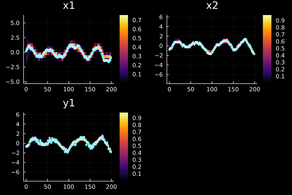

u ad y are then assumed to be vectors of vectors. StaticArrays is recommended for maximum performance.

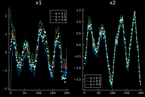
If MonteCarloMeasurements.jl is loaded, you may transform the output particles to Matrix{MonteCarloMeasurements.Particles} with the layout T × n_state using Particles(x,we). Internally, the particles are then resampled such that they all have unit weight. This is conventient for making use of the plotting facilities of MonteCarloMeasurements.jl.

For a full usage example, see the benchmark section below or example_lineargaussian.jl

Resampling

The particle filter will perform a resampling step whenever the distribution of the weights has become degenerate. The resampling is triggered when the effective number of samples is smaller than pf.resample_threshold $\in [0, 1]$, this value can be set when constructing the filter. How the resampling is done is governed by pf.resampling_strategy, we currently provide ResampleSystematic <: ResamplingStrategy as the only implemented strategy. See https://en.wikipedia.org/wiki/Particle_filter for more info.

Particle Smoothing

Smoothing is the process of finding the best state estimate given both past and future data. Smoothing is thus only possible in an offline setting. This package provides a particle smoother, based on forward filtering, backward simulation (FFBS), example usage follows:

N     = 2000 # Number of particles
T     = 80   # Number of time steps
M     = 100  # Number of smoothed backwards trajectories
pf    = ParticleFilter(N, dynamics, measurement, df, dg, d0)
du    = MvNormal(m,1)     # Control input distribution
x,u,y = simulate(pf,T,du) # Simulate trajectory using the model in the filter
tosvec(y) = reinterpret(SVector{length(y[1]),Float64}, reduce(hcat,y))[:] |> copy
x,u,y = tosvec.((x,u,y))

xb,ll = smooth(pf, M, u, y) # Sample smooting particles
xbm   = smoothed_mean(xb)   # Calculate the mean of smoothing trajectories
xbc   = smoothed_cov(xb)    # And covariance
xbt   = smoothed_trajs(xb)  # Get smoothing trajectories
xbs   = [diag(xbc) for xbc in xbc] |> vecvec_to_mat .|> sqrt
plot(xbm', ribbon=2xbs, lab="PF smooth")
plot!(vecvec_to_mat(x), l=:dash, lab="True")

We can plot the particles themselves as well

downsample = 5
plot(vecvec_to_mat(x), l=(4,), layout=(2,1), show=false)
scatter!(xbt[1, 1:downsample:end, :]', subplot=1, show=false, m=(1,:black, 0.5), lab="")
scatter!(xbt[2, 1:downsample:end, :]', subplot=2, m=(1,:black, 0.5), lab="")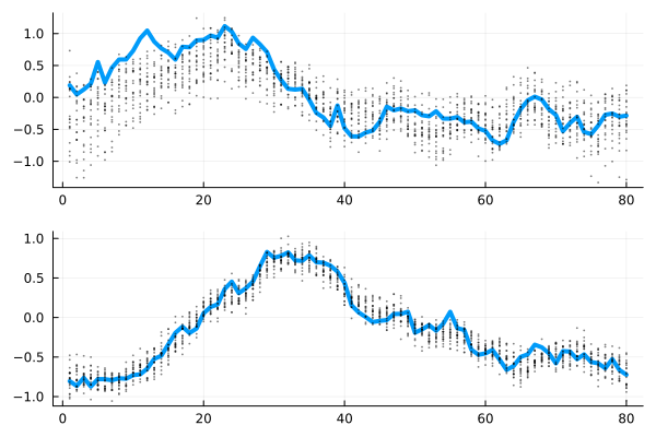

Kalman filter

The KalmanFilter (wiki) assumes that $f$ and $g$ are linear functions, i.e., that they can be written on the form

\[\begin{aligned} x(t+1) &= Ax(t) + Bu(t) + w(t)\\ y(t) &= Cx(t) + Du(t) + e(t) \end{aligned}\]

for some matrices $A,B,C,D$ where $w \sim N(0, R_1)$ and $e \sim N(0, R_2)$ are zero mean and Gaussian. The Kalman filter represents the posterior distributions over $x$ by the mean and a covariance matrix. The magic behind the Kalman filter is that linear transformations of Gaussian distributions remain Gaussian, and we thus have a very efficient way of representing them.

A Kalman filter is easily created using the constructor. Many of the functions defined for particle filters, are defined also for Kalman filters, e.g.:

R1 = cov(df)
R2 = cov(dg)
kf = KalmanFilter(A, B, C, 0, R1, R2, d0)
sol = forward_trajectory(kf, u, y) # filtered, prediction, pred cov, filter cov, loglik

It can also be called in a loop like the pf above

for t = 1:T
    kf(u,y) # Performs both correct and predict!!
    # alternatively
    ll, e = correct!(kf, y, nothing, t) # Returns loglikelihood and prediction error
    x     = state(kf)
    R     = covariance(kf)
    predict!(kf, u, nothing, t)
end

The matrices in the Kalman filter may be time varying, such that A[:, :, t] is $A(t)$. They may also be provided as functions on the form $A(t) = A(x, u, p, t)$. This works for both dynamics and covariance matrices.

The numeric type used in the Kalman filter is determined from the mean of the initial state distribution, so make sure that this has the correct type if you intend to use, e.g., Float32 or ForwardDiff.Dual for automatic differentiation.

Smoothing using KF

Kalman filters can also be used for smoothing

kf = KalmanFilter(A, B, C, 0, cov(df), cov(dg), d0)
xT,R,lls = smooth(kf, u, y, p) # Smoothed state, smoothed cov, loglik

Plot and compare PF and KF

plot(vecvec_to_mat(xT), lab="Kalman smooth", layout=2)
plot!(xbm', lab="pf smooth")
plot!(vecvec_to_mat(x), lab="true")

Kalman filter tuning tutorial

The tutorial "How to tune a Kalman filter" details how to figure out appropriate covariance matrices for the Kalman filter, as well as how to add disturbance models to the system model.

Unscented Kalman Filter

The UnscentedKalmanFilter represents posterior distributions over $x$ as Gaussian distributions, but propagate them through a nonlinear function $f$ by a deterministic sampling of a small number of particles called sigma points (this is referred to as the unscented transform). This UKF thus handles nonlinear functions $f,g$, but only Gaussian disturbances and unimodal posteriors.

The UKF takes the same arguments as a regular KalmanFilter, but the matrices defining the dynamics are replaced by two functions, dynamics and measurement, working in the same way as for the ParticleFilter above.

ukf = UnscentedKalmanFilter(dynamics, measurement, cov(df), cov(dg), MvNormal([1.,1.]), nu=m, ny=p)

UnscentedKalmanFilter{typeof(Main.dynamics), typeof(Main.measurement), Matrix{Float64}, Matrix{Float64}, Distributions.ZeroMeanDiagNormal{Tuple{Base.OneTo{Int64}}}, StaticArraysCore.SVector{2, Float64}, Vector{Float64}, Matrix{Float64}, SciMLBase.NullParameters}
  dynamics: dynamics (function of type typeof(Main.dynamics))
  measurement: measurement (function of type typeof(Main.measurement))
  R1: Array{Float64}((2, 2)) [1.0 0.0; 0.0 1.0]
  R2: Array{Float64}((1, 1)) [1.0;;]
  d0: Distributions.ZeroMeanDiagNormal{Tuple{Base.OneTo{Int64}}}
  xs: Array{StaticArraysCore.SVector{2, Float64}}((5,))
  x: Array{Float64}((2,)) [0.0, 0.0]
  R: Array{Float64}((2, 2)) [1.0 0.0; 0.0 1.0]
  t: Base.RefValue{Int64}
  ny: Int64 1
  nu: Int64 1
  p: SciMLBase.NullParameters SciMLBase.NullParameters()

UKF for DAE systems

See the docstring for DAEUnscentedKalmanFilter or the test file. This filter is modeled after

"Nonlinear State Estimation of Differential Algebraic Systems" Ravi K. Mandela, Raghunathan Rengaswamy, Shankar Narasimhan

Extended Kalman Filter

The ExtendedKalmanFilter (EKF) is similar to the UKF, but propagates Gaussian distributions by linearizing the dynamics and using the formulas for linear systems similar to the standard Kalman filter. This can be slightly faster than the UKF (not always), but also less accurate for strongly nonlinear systems. The linearization is performed automatically using ForwardDiff.jl. In general, the UKF is recommended over the EKF unless the EKF is faster and computational performance is the top priority.

The EKF constructor has the following two signatures

ExtendedKalmanFilter(dynamics, measurement, R1,R2,d0=MvNormal(Matrix(R1)); nu::Int, p = SciMLBase.NullParameters(), α = 1.0, check = true)
ExtendedKalmanFilter(kf, dynamics, measurement)

The first constructor takes all the arguments required to initialize the extended Kalman filter, while the second one takes an already defined standard Kalman filter. using the first constructor, the user must provide the number of inputs to the system, nu.

where kf is a standard KalmanFilter from which the covariance properties are taken.

AdvancedParticleFilter

The AdvancedParticleFilter works very much like the ParticleFilter, but admits more flexibility in its noise models.

The AdvancedParticleFilter type requires you to implement the same functions as the regular ParticleFilter, but in this case you also need to handle sampling from the noise distributions yourself. The function dynamics must have a method signature like below. It must provide one method that accepts state vector, control vector, parameter, time and noise::Bool that indicates whether or not to add noise to the state. If noise should be added, this should be done inside dynamics An example is given below

using Random
const rng = Random.Xoshiro()
function dynamics(x, u, p, t, noise=false) # It's important that this defaults to false
    x = A*x .+ B*u # A simple linear dynamics model in discrete time
    if noise
        x += rand(rng, df) # it's faster to supply your own rng
    end
    x
end

The measurement_likelihood function must have a method accepting state, input, measurement, parameter and time, and returning the log-likelihood of the measurement given the state, a simple example below:

function measurement_likelihood(x, u, y, p, t)
    logpdf(dg, C*x-y) # A simple linear measurement model with normal additive noise
end

This gives you very high flexibility. The noise model in either function can, for instance, be a function of the state, something that is not possible for the simple ParticleFilter. To be able to simulate the AdvancedParticleFilter like we did with the simple filter above, the measurement method with the signature measurement(x,u,p,t,noise=false) must be available and return a sample measurement given state (and possibly time). For our example measurement model above, this would look like this

measurement(x, u, p, t, noise=false) = C*x + noise*rand(rng, dg)

We now create the AdvancedParticleFilter and use it in the same way as the other filters:

apf = AdvancedParticleFilter(N, dynamics, measurement, measurement_likelihood, df, d0)
sol = forward_trajectory(apf, u, y, p)

LowLevelParticleFilters.ParticleFilteringSolution{AdvancedParticleFilter{PFstate{StaticArraysCore.SVector{2, Float64}, Float64}, typeof(Main.dynamics), typeof(Main.measurement), typeof(Main.measurement_likelihood), Distributions.ZeroMeanIsoNormal{Tuple{Base.OneTo{Int64}}}, Distributions.IsoNormal, DataType, Random.Xoshiro, SciMLBase.NullParameters}, Vector{StaticArraysCore.SVector{1, Float64}}, Vector{StaticArraysCore.SVector{1, Float64}}, Matrix{StaticArraysCore.SVector{2, Float64}}, Matrix{Float64}, Matrix{Float64}, Float64}(AdvancedParticleFilter{PFstate{StaticArraysCore.SVector{2, Float64}, Float64}, typeof(Main.dynamics), typeof(Main.measurement), typeof(Main.measurement_likelihood), Distributions.ZeroMeanIsoNormal{Tuple{Base.OneTo{Int64}}}, Distributions.IsoNormal, DataType, Random.Xoshiro, SciMLBase.NullParameters}
  state: PFstate{StaticArraysCore.SVector{2, Float64}, Float64}
  dynamics: dynamics (function of type typeof(Main.dynamics))
  measurement: measurement (function of type typeof(Main.measurement))
  measurement_likelihood: measurement_likelihood (function of type typeof(Main.measurement_likelihood))
  dynamics_density: Distributions.ZeroMeanIsoNormal{Tuple{Base.OneTo{Int64}}}
  initial_density: Distributions.IsoNormal
  resample_threshold: Float64 0.5
  resampling_strategy: LowLevelParticleFilters.ResampleSystematic <: LowLevelParticleFilters.ResamplingStrategy
  rng: Random.Xoshiro
  p: SciMLBase.NullParameters SciMLBase.NullParameters()
  threads: Bool false
, StaticArraysCore.SVector{1, Float64}[[1.3726525671651035], [-0.19017749241406837], [-0.969135273895609], [1.7990647959686696], [1.1110144385114025], [-0.9594843097039815], [-1.1274239345942698], [-0.5594829762214467], [-2.901558433412519], [0.0013676183829511835]  …  [-0.5454971145686814], [-1.1297171136405466], [0.21014259270827282], [0.48656827054769675], [-1.7551048834406582], [-0.8357342602824859], [-0.8014046010265261], [0.1908722396892745], [-0.5053337913476942], [-2.348147189782665]], StaticArraysCore.SVector{1, Float64}[[-0.44348022803301185], [0.3728902891572107], [1.1618477719183686], [1.2445180959734228], [2.443613320100319], [2.4610231356015], [3.529476525682797], [3.147396533604189], [2.5041237734184207], [0.4595294383675411]  …  [-9.506343949568276], [-8.936725651772154], [-6.109513174174267], [-4.870665990846447], [-2.6442780714593064], [-1.4519600086855868], [0.5468149486544414], [3.1976775234498085], [4.312966232481561], [6.3142083778996625]], StaticArraysCore.SVector{2, Float64}[[2.720428091252547, -3.566769705331012] [4.584635754417116, -3.7470745463511905] … [4.886914676634061, 1.8016023033506723] [4.375438432450081, 1.8422697553727208]; [0.6077285335633166, -2.7414808737005782] [0.8499912823022506, -3.0533294822402697] … [3.504556760644718, 3.052191757886864] [3.0592515929979216, 1.8347448141022262]; … ; [3.5014791134498013, 1.0154308045546139] [3.237771289913931, 0.918096002083673] … [4.927224352631614, 5.843251527620085] [2.286366247154358, 6.186783410897698]; [2.5691041723735983, -2.5145320434272707] [2.718309310149591, -3.0796895045578427] … [4.251917738589702, 7.198311724962507] [5.0770885437367514, 9.188456892456111]], [-11.660784696534883 -19.537646725556996 … -9.985379777157707 -18.979607634958505; -9.423719600778949 -14.683017467845676 … -7.626681522782607 -16.65458876845374; … ; -7.847526817537621 -7.385958358350674 … -8.00279192714644 -7.006020824230884; -8.927943928058603 -14.277904450152572 … -10.994514690377898 -14.120277288069591], [8.6255252656595e-6 3.272712367883064e-9 … 4.606856272405245e-5 5.7182236244187005e-9; 8.078497192370569e-5 4.1999733629424207e-7 … 0.00048727518991398803 5.847954696018613e-8; … ; 0.00039071708895316954 0.0006198962960501258 … 0.00033452734691078183 0.0009064081794082653; 0.0001326304421095006 6.297742279316558e-7 … 1.679356651592775e-5 7.372953431403275e-7], -165.68938023252548)

plot(sol, xreal=x)

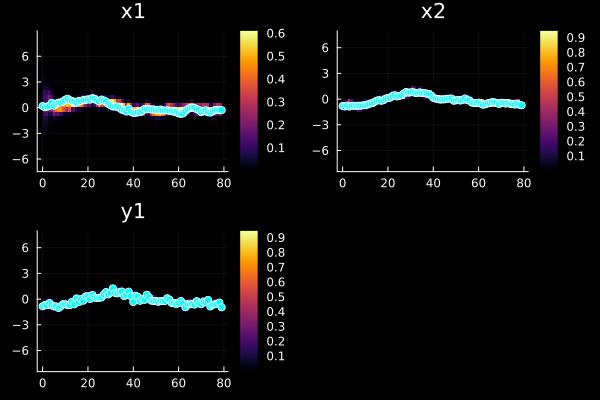
We can even use this type as an AuxiliaryParticleFilter

apfa = AuxiliaryParticleFilter(apf)
sol = forward_trajectory(apfa, u, y, p)
plot(sol, dim=1, xreal=x) # Same as above, but only plots a single dimension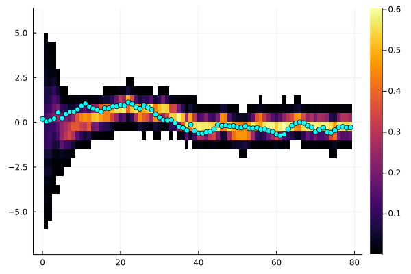

See the tutorials section for more advanced examples, including state estimation for DAE (Differential-Algebraic Equation) systems.

Troubleshooting and tuning

Tuning a particle filter can be quite the challenge. To assist with this, we provide som visualization tools

debugplot(pf,u[1:20],y[1:20], runall=true, xreal=x[1:20])

Time     Surviving    Effective nbr of particles
--------------------------------------------------------------
t:     1   1.000    2000.0
t:     2   1.000    1173.6
t:     3   1.000     774.6
t:     4   1.000     501.4
t:     5   1.000     362.9
t:     6   1.000     210.2
t:     7   0.173    2000.0
t:     8   1.000    1306.5
t:     9   1.000     978.7
t:    10   1.000     691.1
t:    11   1.000     264.7
t:    12   0.208    2000.0
t:    13   1.000    1031.9
t:    14   1.000     759.7
t:    15   1.000     516.7
t:    16   1.000     357.6
t:    17   1.000     234.0
t:    18   0.187    2000.0
t:    19   1.000    1469.8
t:    20   1.000     845.8
GKS: Ghostscript support not compiled in

The plot displays all states and all measurements. The heatmap in the background represents the weighted particle distributions per time step. For the measurement sequences, the heatmap represent the distributions of predicted measurements. The blue dots corresponds to measured values. In this case, we simulated the data and we had access to states as well, if we do not have that, just omit xreal. You can also manually step through the time-series using

• commandplot(pf,u,y; kwargs...)

For options to the debug plots, see ?pplot.

Something seems to be off with this figure as the hottest spot is not really where we would expect it

Optimization of the log likelihood can be done by, e.g., global/black box methods, see BlackBoxOptim.jl, see examples in Parameter Estimation. Standard tricks apply, such as performing the parameter search in log-space etc.