Smoothing the track of a moving beetle

This is an example of smoothing the 2-dimensional trajectory of a moving dung beetle. The example spurred off of this Discourse topic. For more information about the research behind this example, see Artificial light disrupts dung beetles’ sense of direction and A dung beetle that path integrates without the use of landmarks. Special thanks to Yakir Gagnon for providing this example.

In this example we will describe the position coordinates, $x$ and $y$, of the beetle as functions of its velocity, $v_t$, and direction, $θ_t$:

\[\begin{aligned} x_{t+1} &= x_t + \cos(θ_t)v_t \\ y_{t+1} &= y_t + \sin(θ_t)v_t \\ v_{t+1} &= v_t + e_t \\ θ_{t+1} &= θ_t + w_t \end{aligned}\]

where $e_t ∼ N(0,σ_e), w_t ∼ N(0,σ_w)$ The beetle further has two "modes", one where it's moving towards a goal, and one where it's searching in a more erratic manner. Figuring out when this mode switch occurs is the goal of the filtering. The mode will be encoded as a state variable, and used to determine the amount of dynamic noise affecting the velocity of the beetle, i.e., in the searching mode, the beetle has more velocity noise. The mode switching is modeled as a stochastic process with a binomial distribution (coin flip) describing the likelihood of a switch from mode 0 (moving to goal) and mode 1 (searching). Once the beetle has started searching, it stays in that mode, i.e., the searching mode is "sticky" or "terminal".

We load a single experiment from file for the purpose of this example (in practice, there may be hundreds of experiments)

using LowLevelParticleFilters, LinearAlgebra, StaticArrays, Distributions, Plots, Random
using DelimitedFiles
path = "../track.csv"
xyt = readdlm(path)
tosvec(y) = reinterpret(SVector{length(y[1]),Float64}, reduce(hcat,y))[:] |> copy # helper function
y = tosvec(collect(eachrow(xyt[:,1:2])))

We then define some properties of the dynamics and the filter. We will use an AdvancedParticleFilter since we want to have fine-grained control over the noise sampling for the mode switch.

N = 2000 # Number of particles in the particle filter
n = 4 # Dimension of state: we have speed and angle, so two
p = 2 # Dimension of measurements, we can measure the x and the y, so also two
@inline pos(s) = s[SVector(1,2)]
@inline vel(s) = s[3]
@inline ϕ(s) = s[4]
@inline mode(s) = s[5]

We then define the probability distributions we need.

dgσ = 1 # the deviation of the measurement noise distribution
dvσ = 0.3 # the deviation of the dynamics noise distribution
ϕσ  = 0.5
const switch_prob = 0.03 # Probability of mode switch
const dg = MvNormal(@SVector(zeros(p)), dgσ^2) # Measurement noise Distribution
const df = LowLevelParticleFilters.TupleProduct((Normal.(0,[1e-1, 1e-1, dvσ, ϕσ])...,Binomial(1,switch_prob)))
const d0 = MvNormal(SVector(y[1]..., 0.5, atan((y[2]-y[1])...), 0), [3.,3,2,2,0])
const noisevec = zeros(5) # cache vector

We now define the dynamics, since we use the advanced filter, we include the noise=false argument. The dynamics is directly defined in discrete time.

@inline function dynamics(s,u,p,t,noise=false)
    # current state
    m = mode(s)
    v = vel(s)
    a = ϕ(s)
    p = pos(s)
    # get noise
    if noise
        y_noise, x_noise, v_noise, ϕ_noise,_ = rand!(df, noisevec)
    else
        y_noise, x_noise, v_noise, ϕ_noise = 0.,0.,0.,0.
    end
    # next state
    v⁺ = max(0.999v + v_noise, 0.0)
    m⁺ = Float64(m == 0 ? rand() < switch_prob : true)
    a⁺ = a + (ϕ_noise*(1 + m*10))/(1 + v) # next state velocity is used here
    p⁺ = p + SVector(y_noise, x_noise) + SVector(sincos(a))*v # current angle but next velocity
    SVector{5,Float64}(p⁺[1], p⁺[2], v⁺, a⁺, m⁺) # all next state
end
function measurement_likelihood(s,u,y,p,t)
    logpdf(dg, pos(s)-y) # A simple linear measurement model with normal additive noise
end
@inline measurement(s,u,p,t,noise=false) = s[SVector(1,2)] + noise*rand(dg) # We observer the position coordinates with the measurement

In this example, we have no control inputs, we thus define a vector of only zeros. We then solve the forward filtering problem and plot the results.

u = zeros(length(y))
pf = AuxiliaryParticleFilter(AdvancedParticleFilter(N, dynamics, measurement, measurement_likelihood, df, d0))
T = length(y)
sol = forward_trajectory(pf,u[1:T],y[1:T])
(; x,w,we,ll) = sol
plot(sol, markerstrokecolor=:auto, m=(2,0.5)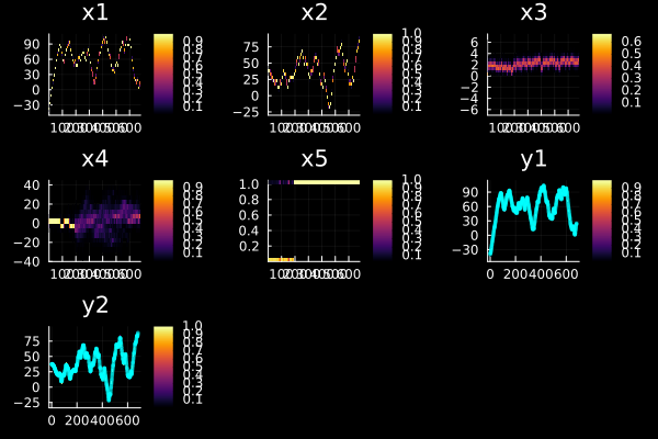, format=:png)

We can clearly see when the beetle switched mode (state variable 5). This corresponds well to annotations provided by a biologist and is the fundamental question we want to answer with the filtering procedure.

We can plot the mean of the filtered trajectory as well

xh = mean_trajectory(x,we)

"plotting helper function"
function to1series(x::AbstractVector, y)
    r,c = size(y)
    y2 = vec([y; fill(Inf, 1, c)])
    x2 = repeat([x; Inf], c)
    x2,y2
end
to1series(y) = to1series(1:size(y,1),y)

fig1 = plot(xh[:,1],xh[:,2], c=:blue, lab="estimate", legend=:bottomleft)
plot!(xyt[:,1],xyt[:,2], c=:red, lab="measurement")

as well as the angle state variable (we subsample the particles to not get sluggish plots)

fig2 = scatter(to1series(ϕ.(x)'[:,1:5:end])..., m=(:black, 0.03, 2), lab="", size=(500,300), format=:png)
plot!(identity.(xh[:,4]), lab="Filtered angle", legend=:topleft, ylims=(-30, 70))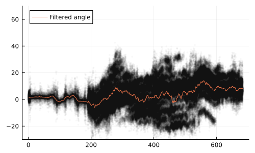

The particle plot above indicate that the posterior is multimodal. This phenomenon arises due to the simple model that uses an angle that is allowed to leave the interval `0-2\pi rad. In this example, we are not interested in the angle, but rather when the beetle switches mode. The filtering distribution above gives a hint at when this happens, but we will not plot the mode trajectory until we have explored smoothing as well.

Smoothing

The filtering results above does not use all the available information when trying to figure out the state trajectory. To do this, we may call a smoother. We use a particle smoother and compute 10 smoothing trajectories.

M = 10 # Number of smoothing trajectories, NOTE: if this is set higher, the result will be better at the expense of linear scaling of the computational cost.
sb,ll = smooth(pf, M, u, y) # Sample smooting particles (b for backward-trajectory)
sbm = smoothed_mean(sb)     # Calculate the mean of smoothing trajectories
sbt = smoothed_trajs(sb)    # Get smoothing trajectories
plot!(fig1, sbm[1,:],sbm[2,:], lab="xs")

plot!(fig2, identity.(sbm'[:,4]), lab="smoothed")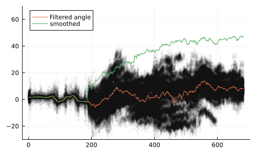

We see that the smoothed trajectory may look very different from the filter trajectory. This is an indication that it's hard to tell what state the beetle is currently in, but easier to look back and tell what state the beetle must have been in at a historical point.

We can also visualize the mode state

plot(xh[:,5], lab="Filtering")
plot!(to1series(sbt[5,:,:]')..., lab="Smoothing", title="Mode trajectories", l=(:black,0.2))

also this state variable indicates that it's hard to tell what state the beetle is in during filtering, but obvious with hindsight (smoothing). The mode switch occurs when the filtering distribution of the angle becomes drastically wider, indicating that increased dynamics noise is required in order to describe the motion of the beetle.

Summary

This example has demonstrated filtering and smoothing in an advanced application that includes manual control over noise, mixed continuous and discrete state.