Benchmarks
Particle filtering
To see how the performance varies with the number of particles, we simulate several times. The following code simulates the system and performs filtering using the simulated measurements. We do this for varying number of time steps and varying number of particles.
function run_test()
    particle_count = [10, 20, 50, 100, 200, 500, 1000]
    time_steps = [20, 100, 200]
    RMSE = zeros(length(particle_count),length(time_steps)) # Store the RMS errors
    propagated_particles = 0
    t = @elapsed for (Ti,T) = enumerate(time_steps)
        for (Ni,N) = enumerate(particle_count)
            montecarlo_runs = 2*maximum(particle_count)*maximum(time_steps) ÷ T ÷ N
            E = sum(1:montecarlo_runs) do mc_run
                pf = ParticleFilter(N, dynamics, measurement, df, dg, d0) # Create filter
                u = @SVector randn(2)
                x = SVector{2,Float64}(rand(rng, d0))
                y = SVector{2,Float64}(sample_measurement(pf,x,u,0,1))
                error = 0.0
                @inbounds for t = 1:T-1
                    pf(u, y) # Update the particle filter
                    x = dynamics(x,u,t) + SVector{2,Float64}(rand(rng, df)) # Simulate the true dynamics and add some noise
                    y = SVector{2,Float64}(sample_measurement(pf,x,u,0,t)) # Simulate a measuerment
                    u = @SVector randn(2) # draw a random control input
                    error += sum(abs2,x-weighted_mean(pf))
                end # t
                √(error/T)
            end # MC
            RMSE[Ni,Ti] = E/montecarlo_runs
            propagated_particles += montecarlo_runs*N*T
            @show N
        end # N
        @show T
    end # T
    println("Propagated $propagated_particles particles in $t seconds for an average of $(propagated_particles/t/1000) particles per millisecond")
    return RMSE
end

@time RMSE = run_test()
Propagated 8400000 particles in 1.140468043 seconds for an average of 7365.397085484139 particles per millisecond
We then plot the results
time_steps     = [20, 100, 200]
particle_count = [10, 20, 50, 100, 200, 500, 1000]
nT             = length(time_steps)
leg            = reshape(["$(time_steps[i]) time steps" for i = 1:nT], 1,:)
plot(particle_count,RMSE,xscale=:log10, ylabel="RMS errors", xlabel=" Number of particles", lab=leg)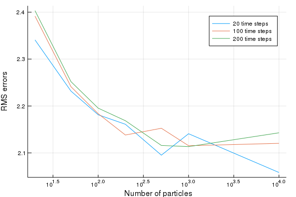
Comparison against filterpy
filterpy is a popular Python library for state estimation. Below, we compare performance on their UKF example, but we use a longer trajectory of 50k time steps:
Python implementation
from filterpy import *
from filterpy.kalman import *
import numpy as np
from numpy.random import randn
from filterpy.common import Q_discrete_white_noise
import time
def fx(x, dt):
    # state transition function - predict next state based
    # on constant velocity model x = vt + x_0
    F = np.array([[1, dt, 0, 0],
                  [0, 1, 0, 0],
                  [0, 0, 1, dt],
                  [0, 0, 0, 1]], dtype=float)
    return np.dot(F, x)

def hx(x):
   # measurement function - convert state into a measurement
   # where measurements are [x_pos, y_pos]
   return np.array([x[0], x[2]])

dt = 0.1
# create sigma points to use in the filter. This is standard for Gaussian processes
points = MerweScaledSigmaPoints(4, alpha=.1, beta=2., kappa=-1)

kf = UnscentedKalmanFilter(dim_x=4, dim_z=2, dt=dt, fx=fx, hx=hx, points=points)
kf.x = np.array([-1., 1., -1., 1]) # initial state
kf.P *= 0.2 # initial uncertainty
z_std = 0.1
kf.R = np.diag([z_std**2, z_std**2]) # 1 standard
kf.Q = Q_discrete_white_noise(dim=2, dt=dt, var=0.01**2, block_size=2)

zs = [[i+randn()*z_std, i+randn()*z_std] for i in range(50000)] # measurements

start_time = time.time()

for z in zs:
    kf.predict()
    kf.update(z)
    # print(kf.x, 'log-likelihood', kf.log_likelihood)

end_time = time.time()
print(f"Execution time: {end_time - start_time} seconds")
Execution time: 6.390492916107178 secondsJulia implementation
using LowLevelParticleFilters, StaticArrays, LinearAlgebra, BenchmarkTools
const dt = 0.1
function fx(x,u,p,t)
    # state transition function - predict next state based
    # on constant velocity model x = vt + x_0
    F = SA[1.0 dt 0.0 0.0;
         0.0 1.0 0.0 0.0;
         0.0 0.0 1.0 dt;
         0.0 0.0 0.0 1.0]
    return F*x
end

function hx(x,u,p,t)
    # measurement function - convert state into a measurement
    # where measurements are [x_pos, y_pos]
    return x[SA[1,3]]
end

x0 = SA[-1.0, 1.0, -1.0, 1.0] # initial state
R0 = 0.2I(4) # initial uncertainty
z_std = 0.1
R1 = LowLevelParticleFilters.double_integrator_covariance(dt, 0.01^2)
R1 = SMatrix{4,4}(cat(R1, R1, dims=(1,2)))  # Called Q in the Python code
R2 = Diagonal(SA[z_std^2, z_std^2])         # Called R in the Python code
d0 = LowLevelParticleFilters.SimpleMvNormal(x0, R0)
ukf = UnscentedKalmanFilter(fx, hx, R1, R2, d0; nu=0, ny=2, Ts=dt, p=nothing)
zs = [[i+randn()*z_std, i+randn()*z_std] for i in 1:50000] # measurements

function runsim(ukf, zs)
    for z in zs
        predict!(ukf, SA[])
        ll, _ = correct!(ukf, SA[], z)
        # @show ll
    end
end

runsim(ukf, zs)

time_julia = @belapsed runsim($ukf, $zs)0.017676814Result
time_python = 6.390492916107178
time_python / time_julia361.51836615507625The Julia version is about 360x faster than the Python version.