Transfer-function estimation using spectral techniques

Frequency-domain estimation refers to estimation of linear systems using frequency-domain data. We distinguish between nonparametric and parametric models, where parametric models have a fixed number of parameters (such as transfer functions with polynomials or statespace models), whereas nonparametric models are typically given as vectors of frequency-response values over a grid of frequencies, i.e., the number of parameters is not fixed and grows with the number of data points.

Nonparametric estimation

Non-parametric estimation refers to the estimation of a model without a fixed number of parameters. Instead, the number of estimated parameters typically grows with the size of the data. This form of estimation can be useful to gain an initial understanding of the system, before selecting model orders etc. for a more standard parametric model. We provide non-parametric estimation of transfer functions through spectral estimation. To illustrate, we once again simulate some data:

using ControlSystemIdentification, ControlSystemsBase, Plots
T          = 100000
h          = 1
sim(sys,u) = lsim(sys, u, 1:T)[1][:]
σy         = 0.5
sys        = tf(1,[1,2*0.1,0.1])
ωn         = sqrt(0.3)
sysn       = tf(σy*ωn,[1,2*0.1*ωn,ωn^2])

u  = randn(1, T)
y  = sim(sys, u)
yn = y + sim(sysn, randn(size(u))) # Add noise filtered through sysn
d  = iddata(y,u,h)
dn = iddata(yn,u,h)

InputOutput data of length 100000, 1 outputs, 1 inputs, Ts = 1

We can now estimate the coherence function to get a feel for whether or nor our data seems to be generated by a linear system:

k = coherence(d)  # Should be close to 1 if the system is linear and noise free
k = coherence(dn) # Slightly lower values are obtained if the system is subject to measurement noise

We can also estimate a transfer function using spectral techniques, the main entry point to this is the function tfest, which returns a transfer-function estimate and an estimate of the power-spectral density of the noise (note, the unit of the PSD is squared compared to a transfer function, hence the √N when plotting it in the code below):

G,N = tfest(dn)
bodeplot([sys,sysn], exp10.(range(-3, stop=log10(pi), length=200)), layout=(1,3), plotphase=false, subplot=[1,2,2], ylims=(0.1,300), linecolor=:blue)

coherenceplot!(dn, subplot=3)
plot!(G, subplot=1, lab="G Est", alpha=0.3, title="Process model")
plot!(√N, subplot=2, lab="N Est", alpha=0.3, title="Noise model")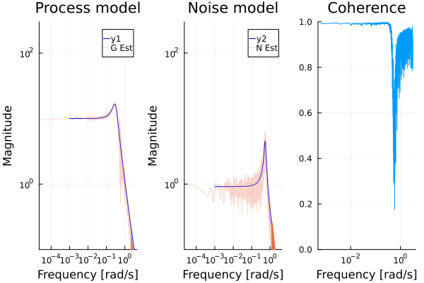

The left figure displays the Bode magnitude of the true system, together with the estimate (noisy), and the middle figure illustrates the estimated noise model. The right figure displays the coherence function (coherenceplot), which is close to 1 everywhere except for at the resonance peak of the noise log10(sqrt(0.3)) = -0.26.

See the example notebooks for more details.

Parametric estimation

Transfer functions

To estimate a parametric, rational transfer function from frequency-domain data, call tfest with an FRD object and an initial guess for the system model. This initial guess determines the number of coefficients in the numerator and denominator of the estimated model.

G0 = tf(1.0, [1,1,1]) # Initial guess
G = tfest(d::FRD, G0)

Internally, Optim is using a gradient-based optimizer to find the optimal fit of the bode curve of the system. The default optimizer BFGS can be changed, see the docstring ?tfest.

For a comparison between estimation in the time and frequency domains, see this notebook.

If the above problem is hard to solve, you may parametrize the model using, e.g., a Laguerre basis expansion, example:

basis = laguerre_oo(1, 50) # Use 50 basis functions, the final model order may be reduced with baltrunc
Gest,p = tfest(d::FRD, basis)

Note

Most methods for frequency-domain estimation of transfer functions handle SISO or SIMO systems only. For estimation of MIMO systems, consider using state-space based methods and convert the result to a transfer function using tf after estimation if required.

Statespace

The function subspaceid handles frequency-domain data (as well as time-domain data). If an InputOutputFreqData is passed (may be created with function iddata), a frequency-domain method is automatically used. Further, a frequency-response object, FRD, may also be passed, in which case it is transformed to an InputOutputFreqData automatically. If the frequency-response data stems from a frequency-response analysis, you may need to perform a bilinear transform on the frequency axis of the data object to convert the continuous-time frequency axis to discrete time, example:

Ts    = 0.01 # Sample time
frd_d = c2d(frd_c::FRD, Ts) # Perform a bilinear transformation to discrete-time frequency vector
Ph, _ = subspaceid(frd_d, Ts, nx)

This can be done automatically by passing bilinear_transform = true to subspaceid.

The following example generates simulated frequency-response data frd from a random system, this data could in practice have come from a frequency-response analysis. We then use the data to fit a model using subspace-based identification in the frequency domain using subspaceid.

using ControlSystemIdentification, ControlSystemsBase, Plots
ny,nu,nx = 2,3,5                        # number of outputs, inputs and states
Ts = 1                                  # Sample time
G = ssrand(ny,nu,nx; Ts, proper=true)   # Generate a random system

N = 200             # Number of frequency points
w = freqvec(Ts, N)
frd = FRD(w, G)     # Build a frequency-response data object (this should in practice come from an experiment)

Gh, x0 = subspaceid(frd, G.Ts, nx; zeroD=true) # Fit frequency response
sigmaplot([G, Gh], w[2:end], lab=["True system" "Estimated model"])

Model-based spectral estimation

The model estimation procedures can be used to estimate spectrograms. This package extends some methods from DSP.jl to accept a estimation function as the second argument. To create a suitable such function, we provide the function model_spectrum. Usage is illustrated below.

using ControlSystemIdentification, DSP
T  = 1000
fs = 1
s = sin.((1:1/fs:T) .* 2pi/10) + 0.5randn(T)
S1 = spectrogram(s,window=hanning, fs=fs)            # Standard spectrogram
estimator = model_spectrum(ar,1/fs,6)
S2 = spectrogram(s,estimator,window=rect, fs=fs)     # Model-based spectrogram
plot(plot(S1,title="Standard Spectrogram"),plot(S2,title="AR Spectrogram")) # Requires the package LPVSpectral.jl

window

ControlSystemIdentification.tfest — Function

H, N = tfest(data, σ = 0.05, method = :corr)

Estimate a transfer function model using the Correlogram approach (default) using the signal model $y = H(iω)u + n$.

Both H and N are of type FRD (frequency-response data).

σ determines the width of the Gaussian window applied to the estimated correlation functions before FFT. A larger σ implies less smoothing.
H = Syu/Suu Process transfer function
N = Sy - |Syu|²/Suu Estimated Noise PSD (also an estimate of the variance of $H$). Note that a PSD is related to the "noise model" $N_m$ used in the system identification literature as $N_{psd} = N_m^* N_m$. The magnitude curve of the noise model can be visualized by plotting √(N).
method: :welch or :corr. :welch uses the Welch method to estimate the power spectral density, while :corr (default) uses the Correlogram approach. If method = :welch, the additional keyword arguments n, noverlap and window determine the number of samples per segment (default 10% of data), the number of samples to overlap between segments (default 50%), and the window function to use (default hamming), respectively.

Extended help

This estimation method is unbiased if the input $u$ is uncorrelated with the noise $n$, but is otherwise biased (e.g., for identification in closed loop).

source

tfest(
    data::FRD,
    p0,
    link = log ∘ abs;
    freq_weight = sqrt(data.w[1]*data.w[end]),
    refine = true,
    opt = BFGS(),
    opts = Optim.Options(
        store_trace       = true,
        show_trace        = true,
        show_every        = 1,
        iterations        = 100,
        allow_f_increases = false,
        time_limit        = 100,
        x_tol             = 0,
        f_tol             = 0,
        g_tol             = 1e-8,
        f_calls_limit     = 0,
        g_calls_limit     = 0,
    ),
)

Fit a parametric transfer function to frequency-domain data.

The initial pahse of the optimization solves

\[\operatorname{minimize}_{B,A}{|| B/l - A||}\]

and the second stage (if refine=true) solves

\[\operatorname{minimize}_{B,A}{|| \text{link}\left(\dfrac{B}{A}\right) - \text{link}\left(l\right)||}\]

(abs2(link(B/A) - link(l)))

Arguments:

data: An FRD onbject with frequency domain data.
p0: Initial parameter guess. Can be a NamedTuple or ComponentVector with fields b,a specifying numerator and denominator as they appear in the call to tf, i.e., (b = [1.0], a = [1.0,1.0,1.0]). Can also be an instace of TransferFunction.
link: By default, phase information is discarded in the fitting. To include phase, change to link = log.
freq_weight: Apply weighting with the inverse frequency. The value determines the cutoff frequency before which the weight is constant, after which the weight decreases linearly. Defaults to the geometric mean of the smallest and largest frequency.
refine: Indicate whether or not a second optimization stage is performed to refine the results of the first.
opt: The Optim optimizer to use.
opts: Optim.Options controlling the solver options.

See also minimum_phase to transform a possibly non-minimum phase system to minimum phase.

source

tfest(data::FRD, basis::AbstractStateSpace; 
    freq_weight = 1 ./ (data.w .+ data.w[2]),
    opt = BFGS(),
    metric::M = abs2,
    opts = Optim.Options(
        store_trace       = true,
        show_trace        = true,
        show_every        = 50,
        iterations        = 1000000,
        allow_f_increases = false,
        time_limit        = 100,
        x_tol             = 1e-5,
        f_tol             = 0,
        g_tol             = 1e-8,
        f_calls_limit     = 0,
        g_calls_limit     = 0,
)

Fit a parametric transfer function to frequency-domain data using a pre-specified basis.

Arguments:

data: An FRD onbject with frequency domain data.

function kautz(a::AbstractVector)

basis: A basis for the estimation. See, e.g., laguerre, laguerre_oo, kautz
freq_weight: A vector of weights per frequency. The default is approximately 1/f.
opt: The Optim optimizer to use.
opts: Optim.Options controlling the solver options.

source

ControlSystemIdentification.coherence — Function

κ² = coherence(d; n = length(d)÷10, noverlap = n÷2, window=hamming, method=:welch)

Calculates the magnitude-squared coherence Function. κ² close to 1 indicates a good explainability of energy in the output signal by energy in the input signal. κ² << 1 indicates that either the system is nonlinear, or a strong noise contributes to the output energy.

κ: Squared coherence function in the form of an FRD.
method: :welch or :corr. :welch uses the Welch method to estimate the power spectral density, while :corr uses the Correlogram approach . For method = :corr, the additional keyword argument σ determines the width of the Gaussian window applied to the estimated correlation functions before FFT. A larger σ implies less smoothing.