Statespace model estimation
This page documents the facilities available for estimating linear statespace models with inputs on the form
\[\begin{aligned} x^+ &= Ax + Bu + Ke\\ y &= Cx + Du + e \end{aligned}\]
This package estimates models in discrete time, but they may be converted to continuous-time models using the function d2c from ControlSystemsBase.jl.
There exist several methods for identification of statespace models, subspaceid, n4sid, newpem, structured_pem and era. subspaceid is the most comprehensive algorithm for subspace-based identification whereas n4sid is an older implementation. newpem solves the prediction-error problem using an iterative optimization method (from Optim.jl) and is generally slightly more accurate but also more computationally expensive. While newpem estimates an unstructured model (black box), structured_pem allows you to estimate a statespace model with a predefined structure (gray box). If unsure which method to use, try subspaceid first (unless the data comes from closed-loop operation, use newpem in this case).
Subspace-based identification using n4sid and subspaceid
In this example we will estimate a statespace model using the subspaceid method. This function returns an object of type N4SIDStateSpace where the model is accessed as sys.sys.
using ControlSystemIdentification, ControlSystemsBase, Plots
Ts = 0.1
G  = c2d(DemoSystems.resonant(), Ts)
u  = randn(1,1000)
y  = lsim(G,u).y
y .+= 0.01 .* randn.() # add measurement noise
d  = iddata(y,u,Ts)
sys = subspaceid(d, :auto; verbose=false, zeroD=true)

# or use a robust version of svd if y has outliers or missing values
# using TotalLeastSquares
# sys = n4sid(d, :auto; verbose=false, svd=x->rpca(x)[3])
bodeplot([G, sys.sys], lab=["True" "" "subspace" ""])
N4SIDStateSpace is a subtype of AbstractPredictionStateSpace, a statespace object that contains an observer gain matrix sys.K (Kalman filter) as well as estimated covariance matrices etc.
Using the function n4sid instead, we have
sys2 = n4sid(d, :auto; verbose=false, zeroD=true)
bodeplot!(sys2.sys, lab=["n4sid" ""])
subspaceid allows you to choose the weighting between :MOESP, :CVA, :N4SID, :IVM and is generally preferred over n4sid.
Both functions allow you to choose which functions are used for least-squares estimates and computing the SVD, allowing e.g., robust estimators for resistance against outliers etc.
Tuning the model fit
The subspace-based estimation algorithms have a number of parameters that can be tuned if the initial model fit is not satisfactory.
focusdetermines the focus of the model fit. The default is:predictionwhich minimizes the prediction error. If this choice produces an unstable model for a stable system, or the simmulation performance is poor,focus = :simulationmay be a better choice.- There are several horizon parameters that can be tuned. The keyword argument
rselects the prediction horizon, this has to be greater than the model order, with the default beingnx + 10.s1ands2control the past horizons for the output and input, respectively. The default iss1 = s2 = r. Past horizons can only be tuned forsubspaceid. - (Advanced) The method used to compute the svd as well as performing least-squares fitting can be changed using the keywords
svd, Aestimator, Bestimator. zeroDallows you to force the estimated $D$ matrix to be zero (a strictly proper model).- It is possible to select the weight type
W, choose between:MOESP, :CVA, :N4SID, :IVM. The default is:MOESP.
See the docstrings of subspaceid and n4sid for additional arguments and more details.
ERA and OKID
The "Eigenvalue realization algorithm" and "Observer Kalman identification" algorithms are available as era and okid. If era is called with a data object, okid is automatically used internally to produce the Markov parameters to the ERA algorithm.
sys3 = era(d, 2) # era has a lot of parameters that may require tuning
bodeplot!(sys3, lab=["ERA" ""])
Using multiple datasets
ERA/OKID supports the use of multiple datasets to improve the estimation accuracy. Below, we show how to perform this manually
using ControlSystemIdentification, ControlSystemsBase, Plots, Statistics
Ts = 0.1
G = c2d(tf(1, [1,1,1]), Ts) # True system

# Create several "experiments"
ds = map(1:5) do i
    u = randn(1, 1000)
    y, t, x = lsim(G, u)
    yn = y + 0.2randn(size(y))
    iddata(yn, u, Ts)
end

Ys = okid.(ds, 2, round(Int, 10/Ts), smooth=true, λ=1)    # Estimate impulse response for each experiment
Y = mean(Ys)                            # Average all impulse responses

imp = impulse(G, 10)
f1 = plot(imp, lab="True", l=5)
plot!(imp.t, vec.(Ys), lab="Individual estimates", title="Impulse-response estimates")
plot!(imp.t, vec(Y), l=(3, :black), lab="Mean")

models = era.(Ys, Ts, 2, 50, 50)    # estimate models based on individual experiments
meanmodel = era(Y, Ts, 2, 50, 50)   # estimate model based on mean impulse response

f2 = bodeplot([G, meanmodel], lab=["True" "" "Combined estimate" ""], l=2)
bodeplot!(models, lab="Individual estimates", c=:black, alpha=0.5, legend=:bottomleft)

plot(f1, f2)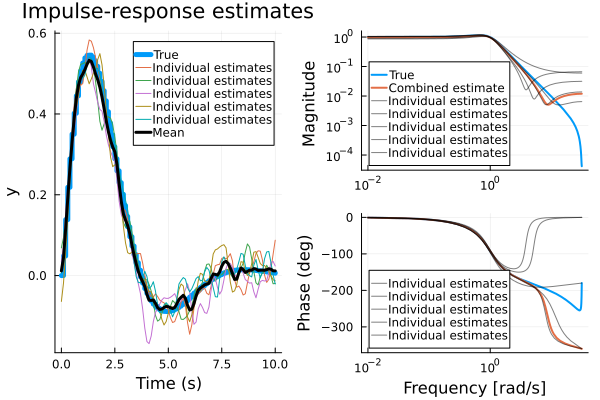
The procedure shown above is equivalent to calling era directly with a vector of data sets, in which case the averaging of the impulse responses is done internally.
era(ds, 2, 50, 50, round(Int, 10/Ts), p=1, λ=1, smooth=true) # Should be identical to meanmodel aboveStateSpace{Discrete{Float64}, Float64}
A =
0.971427881570261 -0.0855584206109082
0.08555842061090893 0.9234421371153649
B =
-0.06557401221406604
0.06270434654177275
C =
-0.6557401221406601 -0.6270434654177278
D =
0.011468386761001372
Sample Time: 0.1 (seconds)
Discrete-time state-space modelPrediction-error method (PEM)
The prediction-error method is a simple but powerful algorithm for identification of discrete-time LTI systems on state-space form:
\[\begin{aligned} x' &= Ax + Bu + Ke \\ y &= Cx + Du + e \end{aligned}\]
The user can choose to minimize either prediction errors or simulation errors, with arbitrary metrics, i.e., not limited to squared errors.
The result of the identification with newpem is a custom type with extra fields for the identified Kalman gain and noise covariance matrices.
Three distinct flavors of PEM exist in this package:
newpem: Linear black-box model estimation (unstructured models)structured_pem: Linear structured model estimation (user-defined structure/gray box)ControlSystemIdentification.nonlinear_pem: Nonlinear gray-box model estimation (e.g., ODE parameter estimation)
Usage example
Below, we generate a system and simulate it forward in time. We then try to estimate a model based on the input and output sequences using the function newpem.
using ControlSystemIdentification, ControlSystemsBase, Random, LinearAlgebra
using ControlSystemIdentification: newpem
sys = c2d(tf(1, [1, 0.5, 1]) * tf(1, [1, 1]), 0.1)

Random.seed!(1)
T   = 1000                      # Number of time steps
nx  = 3                         # Number of poles in the true system
nu  = 1                         # Number of inputs
x0  = randn(nx)                 # Initial state
sim(sys,u,x0=x0) = lsim(ss(sys), u, x0=x0).y # Helper function
u   = randn(nu,T)               # Generate random input
y   = sim(sys, u, x0)           # Simulate system
y .+= 0.01 .* randn.()          # Add some measurement noise
d   = iddata(y,u,0.1)

sysh,opt = newpem(d, nx, focus=:prediction) # Estimate model

yh = predict(sysh, d) # Predict using estimated model
predplot(sysh, d)     # Plot prediction and true output
See the example notebooks for more plots as well as several examples in the example section of this documentation.
Arguments
The algorithm has several options:
- The optimization is by default started with an initial guess provided by
subspaceid, but this can be overridden by providing an initial guess tonewpemusing the keyword argumentsys0. focusdetermines the focus of the model fit. The default is:predictionwhich minimizes the prediction error. If this choice produces an unstable model for a stable system, or the simulation performance is poor,focus = :simulationmay be a better choice.- A regularizer may be provided using the keyword argument
regularizer. - A stable model may be enforced using
stable = true. - The $D$ matrix may be forced to be zero using
zeroD = true. - A trade-off between prediction and simulation performance can be achieved by optimizing the $h$-step prediction error. The default is $h=1$ which corresponds to the standard prediction error. This can be changed using the keyword argument
h. A large value ofhwill make the optimization problem computationally expensive to solve.
See the docstring of newpem for additional arguments and more details.
Internals
Internally, Optim.jl is used to optimize the system parameters, using automatic differentiation to calculate gradients (and Hessians where applicable). Optim solver options can be controlled by passing keyword arguments to newpem, and by passing a manually constructed solver object. The default solver is BFGS()
Gray-box identification
For estimation of linear or nonlinear models with fixed structure, see structured_pem (linear) and ControlSystemIdentification.nonlinear_pem.
Filtering, prediction and simulation
When you estimate models, you can sometimes select the "focus" of the estimation, to either focus on :prediciton performance or :simulation performance. Simulation tends to require accurate low-frequency properties, especially for integrating systems, whereas prediction favors an accurate model for higher frequencies. If there are significant input disturbances affecting the system, or if the system is unstable, prediction focus is generally preferred.
When you validate the estimated models, you can simulate them using lsim from ControlSystemsBase.jl or using simulate. You may also convert the model to a KalmanFilter from LowLevelParticleFilters.jl by calling KalmanFilter(sys), after which you can perform filtering and smoothing etc. with the utilities provided for a KalmanFilter.
Furthermore, we have the utility functions below
predict(sys, d, x0=zeros; h=1): Form predictions using estimatedsys, this essentially runs a stationary Kalman filter.hdenotes the prediction horizon.simulate(sys, u, x0=zeros): Simulate the system using inputu. The noise model and Kalman gain does not have any influence on the simulated output.observer_predictor: Extract the predictor model from the estimated system (ss(A-KC,[B K],C,D)).observer_controllerprediction_errorprediction_error_filterpredictiondatanoise_model
Code generation
To generate C-code for, e.g., simulating a system, see SymbolicControlSystems.jl.
Statespace API
ControlSystemIdentification.eraControlSystemIdentification.n4sidControlSystemIdentification.newpemControlSystemIdentification.noise_modelControlSystemIdentification.okidControlSystemIdentification.prediction_errorControlSystemIdentification.prediction_error_filterControlSystemIdentification.structured_pemControlSystemIdentification.subspaceidControlSystemsBase.observer_controllerControlSystemsBase.observer_predictor
ControlSystemIdentification.newpem — Function
sys, x0, res = newpem(
    d,
    nx;
    zeroD  = true,
    focus  = :prediction,
    h      = 1,
    stable = true,
    sys0   = subspaceid(d, nx; zeroD, focus, stable),
    metric = abs2,
    regularizer = (p, P) -> 0,
    output_nonlinearity = nothing,
    input_nonlinearity = nothing,
    nlp = nothing,
    optimizer = BFGS(
        linesearch = LineSearches.BackTracking(),
    ),
    autodiff = AutoForwardDiff(),
    store_trace = true,
    show_trace  = true,
    show_every  = 50,
    iterations  = 10000,
    time_limit  = 100,
    x_tol       = 0,
    f_abstol    = 0,
    g_tol       = 1e-12,
    f_calls_limit = 0,
    g_calls_limit = 0,
    allow_f_increases = false,
)
A new implementation of the prediction-error method (PEM). Note that this is an experimental implementation and subject to breaking changes not respecting semver.
The prediction-error method is an iterative, gradient-based optimization problem, as such, it can be extra sensitive to signal scaling, and it's recommended to perform scaling to d before estimation, e.g., by pre and post-multiplying with diagonal matrices d̃ = Dy*d*Du, and apply the inverse scaling to the resulting system. In this case, we have
\[D_y y = G̃ D_u u ↔ y = D_y^{-1} G̃ D_u u\]
hence G = Dy \ G̃ * Du where $ G̃ $ is the plant estimated for the scaled iddata. Example:
Dy = Diagonal(1 ./ vec(std(d.y, dims=2))) # Normalize variance
Du = Diagonal(1 ./ vec(std(d.u, dims=2))) # Normalize variance
d̃ = Dy * d * Du
If a manually provided initial guess sys0, this must also be scaled appropriately.
Arguments:
d:iddatanx: Model orderzeroD: Force zeroDmatrixstableif true, stability of the estimated system will be enforced by eigenvalue reflection usingschur_stabwithϵ=1/100(default). Ifstableis a real value, the value is used instead of the defaultϵ.sys0: Initial guess, if non provided,subspaceidis used as initial guess.focus:predictionor:simulation. If:simulation, theKmatrix will be zero.h: Prediction horizon for the prediction error filter. Large values ofhmakes the problem computationally expensive. Ashapproaches infinity, the problem approaches thefocus = :simulationcase.optimizer: One of Optim's optimizersautodiff: Whether or not to use forward-mode AD to compute gradients.AutoForwardDiff()(default) for forward-mode AD, orAutoFiniteDiff()for finite differences.metric: The metric used to measure residuals. Try, e.g.,absfor better resistance to outliers.
The rest of the arguments are related to Optim.Options.
regularizer: A function of the parameter vector and the correspondingPredictionStateSpace/StateSpacesystem that can be used to regularize the estimate.output_nonlinearity: A function of(y::Vector, p)that operates on the output signal at a single time point,yₜ, and modifies it in-place. See below for details.pis a vector of estimated parameters that can be optimized.input_nonlinearity: A function of(u::Matrix, p)that operates on the entire input signaluat once and modifies it in-place. See below for details.pis a vector of estimated parameters that is shared withoutput_nonlinearity.nlp: Initial guess vector for nonlinear parameters. Ifoutput_nonlinearityis provided, this can optionally be provided.
Nonlinear estimation
Nonlinear systems on Hammerstein-Wiener form, i.e., systems with a static input nonlinearity and a static output nonlinearity with a linear system inbetween, can be estimated as long as the nonlinearities are known. The procedure is
- If there is a known input nonlinearity, manually apply the input nonlinearity to the input signal
ubefore estimation, i.e., use the nonlinearly transformed input in theiddataobjectd. If the input nonlinearity has unknown parameters, provide the input nonlinearity as a function using the keyword argumentinput_nonlinearitytonewpem. This function is expected to operate on the entire (matrix) input signaluand modify it in-place. - If the output nonlinearity is invertible, apply the inverse to the output signal
ybefore estimation similar to above. - If the output nonlinearity is not invertible, provide the nonlinear output transformation as a function using the keyword argument
output_nonlinearitytonewpem. This function is expected to operate on the (vector) output signalyand modify it in-place. Example:
function output_nonlinearity(y, p)
    y[1] = y[1] + p[1]*y[1]^2       # Note how the incoming vector is modified in-place
    y[2] = abs(y[2])
end
Please note, y = f(y) does not change y in-place, but creates a new vector y and assigns it to the variable y. This is not what we want here.
The second argument to input_nonlinearity and output_nonlinearity is an (optional) vector of parameters that can be optimized. To use this option, pass the keyword argument nlp to newpem with a vector of initial guesses for the nonlinear parameters. The nonlinear parameters are shared between output and input nonlinearities, i.e., these two functions will receive the same vector of parameters.
The result of this estimation is the linear system without the nonlinearities.
Example
The following simulates data from a linear system and estimates a model. For an example of nonlinear identification, see the documentation.
using ControlSystemIdentification, ControlSystemsBase Plots
G = DemoSystems.doylesat()
T = 1000  # Number of time steps
Ts = 0.01 # Sample time
sys = c2d(G, Ts)
nx = sys.nx
nu = sys.nu
ny = sys.ny
x0 = zeros(nx) # actual initial state
sim(sys, u, x0 = x0) = lsim(sys, u; x0)[1]

σy = 1e-1 # Noise covariance

u  = randn(nu, T)
y  = sim(sys, u, x0)
yn = y .+ σy .* randn.() # Add measurement noise
d  = iddata(yn, u, Ts)

sysh, x0h, opt = ControlSystemIdentification.newpem(d, nx, show_every=10)

plot(
    bodeplot([sys, sysh]),
    predplot(sysh, d, x0h), # Include the estimated initial state in the prediction
)
The returned model is of type PredictionStateSpace and contains the field sys with the system model, as well as covariance matrices and estimated Kalman gain for a Kalman filter.
See also structured_pem and nonlinear_pem.
Extended help
This implementation uses a tridiagonal parametrization of the A-matrix that has been shown to be favourable from an optimization perspective.¹ The initial guess sys0 is automatically transformed to a special tridiagonal modal form. [1]: Mckelvey, Tomas & Helmersson, Anders. (1997). State-space parametrizations of multivariable linear systems using tridiagonal matrix forms.
The parameter vector used in the optimization takes the following form
p = [trivec(A); vec(B); vec(C); vec(D); vec(K); vec(x0)]Where ControlSystemIdentification.trivec vectorizes the -1,0,1 diagonals of A. If focus = :simulation, K is omitted, and if zeroD = true, D is omitted.
ControlSystemIdentification.structured_pem — Function
structured_pem(
    d,
    nx;
    focus = :prediction,
    p0,
    x0 = nothing,
    K0 = focus == :prediction ? zeros(nx, d.ny) : zeros(0,0),
    constructor,
    h = 1,
    metric::F = abs2,
    regularizer::RE = (p, P, simresult) -> 0,
    optimizer = BFGS(
        # alphaguess = LineSearches.InitialStatic(alpha = 0.95),
        linesearch = LineSearches.BackTracking(),
    ),
    store_trace = true,
    show_trace = true,
    show_every = 50,
    iterations = 10000,
    allow_f_increases = false,
    time_limit = 100,
    x_tol = 0,
    f_abstol = 1e-16,
    g_tol = 1e-12,
    f_calls_limit = 0,
    g_calls_limit = 0,
)
Linear gray-box model identification using the prediction-error method (PEM).
This function differs from newpem in that here, the user controls the structure of the estimated model, while in newpem a generic black-box structure is used.
The user provides the function constructor(p) that constructs the model from the parameter vector p. This function must return a statespace system. p0 is the corresponding initial guess for the parameters. K0 is an initial guess for the observer gain (only used if focus = :prediciton) and x0 is the initial guess for the initial condition (estimated automatically if not provided).
For other options, see newpem.
ControlSystemIdentification.subspaceid — Function
subspaceid(
    data::InputOutputData,
    nx = :auto;
    verbose = false,
    r = nx === :auto ? min(length(data) ÷ 20, 50) : nx + 10, # the maximal prediction horizon used
    s1 = r, # number of past outputs
    s2 = r, # number of past inputs
    W = :MOESP,
    zeroD = false,
    stable = true,
    focus = :prediction,
    svd::F1 = svd!,
    scaleU = true,
    Aestimator::F2 = \,
    Bestimator::F3 = \,
    weights = nothing,
)
Estimate a state-space model using subspace-based identification. Several different subspace-based algorithms are available, and can be chosen using the W keyword. Options are :MOESP, :CVA, :N4SID, :IVM.
Ref: Ljung, Theory for the user.
Resistance against outliers can be improved by supplying a custom factorization algorithm and replacing the internal least-squares estimators. See the documentation for the keyword arguments svd, Aestimator, and Bestimator below.
The returned model is of type N4SIDStateSpace and contains the field sys with the system model, as well as covariance matrices for a Kalman filter.
Arguments:
data: Identification dataiddatanx: Rank of the model (model order)verbose: Print stuff?r: Prediction horizon. The model may perform better on simulation if this is made longer, at the expense of more computation time.s1: past horizon of outputss2: past horizon of inputsW: Weight type, choose between:MOESP, :CVA, :N4SID, :IVMzeroD: Force theDmatrix to be zero.stable: Stabilize unstable system using eigenvalue reflection.focus::predictionorsimulationsvd: The function to use forsvd. For resistance against outliers, consider usingTotalLeastSquares.rpcato preprocess the data matrix before applyingsvd, likesvd = A->svd!(rpca(A)[1]).scaleU: Rescale the input channels to have the same energy.Aestimator: Estimator function used to estimateA,C. The default is `, i.e., least squares, but robust estimators, such asirls, flts, rtls` from TotalLeastSquares.jl, can be used to gain resistance against outliers.Bestimator: Estimator function used to estimateB,D. Weighted estimation can be eachieved by passingwlsfrom TotalLeastSquares.jl together with theweightskeyword argument.weights: A vector of weights can be provided if theBestimatoriswls.
Extended help
A more accurate prediciton model can sometimes be obtained using newpem, which is also unbiased for closed-loop data (subspaceid is biased for closed-loop data, see example in the docs). The prediction-error method is iterative and generally more expensive than subspaceid, and uses this function (by default) to form the initial guess for the optimization.
model, x0 = subspaceid(frd::FRD, Ts, args...; estimate_x0 = false, bilinear_transform = false, kwargs...)If a frequency-reponse data object is supplied
- The FRD will be automatically converted to an
InputOutputFreqData estimate_x0is by default set to 0.bilinear_transformtransform the frequency vector to discrete time, see note below.
Note: if the frequency-response data comes from a frequency-response analysis, a bilinear transform of the data is required before estimation. This transform will be applied if bilinear_transform = true.
model, x0 = subspaceid(data::InputOutputFreqData,
    Ts = data.Ts,
    nx = :auto;
    cont = false,
    verbose = false,
    r = nx === :auto ? min(length(data) ÷ 20, 20) : 2nx, # Internal model order
    zeroD = false,
    estimate_x0 = true,
    stable = true,
    svd = svd!,
    Aestimator = \,
    Bestimator = \,
    weights = nothing
)
Estimate a state-space model using subspace-based identification in the frequency domain.
If results are poor, try modifying r, in particular if the amount of data is low.
See the docs for an example.
Arguments:
data: A frequency-domain identification data object.Ts: Sample time at which the data was collectednx: Desired model order, an interer or:auto.cont: Return a continuous-time model? A bilinear transformation is used to convert the estimated discrete-time model, see functiond2c.verbose: Print stuff?r: Internal model order, must be ≥nx.zeroD: Force theDmatrix to be zero.estimate_x0: Esimation of extra parameters to account for initial conditions. This may be required if the data comes from the fft of time-domain data, but may not be required if the data is collected using frequency-response analysis with exactly periodic input and proper handling of transients.stable: For the model to be stable (usesschur_stab).svd: Thesvdfunction to use.Aestimator: The estimator of theAmatrix (and initialC-matrix).Bestimator: The estimator of B/D and C/D matrices.weights: An optional vector of frequency weights of the same length as the number of frequencies in `data.
ControlSystemIdentification.n4sid — Function
res = n4sid(data, r=:auto; verbose=false)Estimate a statespace model using the n4sid method. Returns an object of type N4SIDStateSpace where the model is accessed as res.sys.
Implements the simplified algorithm (alg 2) from "N4SID: Subspace Algorithms for the Identification of Combined Deterministic Stochastic Systems" PETER VAN OVERSCHEE and BART DE MOOR
The frequency weighting is borrowing ideas from "Frequency Weighted Subspace Based System Identification in the Frequency Domain", Tomas McKelvey 1996. In particular, we apply the output frequency weight matrix (Fy) as it appears in eqs. (16)-(18).
Arguments:
data: Identification datadata = iddata(y,u)r: Rank of the model (model order)verbose: Print stuff?Wf: A frequency-domain model of measurement disturbances. To focus the attention of the model on a narrow frequency band, try something likeWf = Bandstop(lower, upper, fs=1/Ts)to indicate that there are disturbances outside this band.i: Algorithm parameter, generally no need to tune thisγ: Set this to a value between (0,1) to stabilize unstable models such that the largest eigenvalue has magnitude γ.zeroD: defaults to false
See also the newer implementation subspaceid which allows you to choose between different weightings (n4sid being one of them). A more accurate prediciton model can sometimes be obtained using newpem, which is also unbiased for closed-loop data.
ControlSystemIdentification.era — Function
era(YY::AbstractArray{<:Any, 3}, Ts, nx::Int, m::Int = 2nx, n::Int = 2nx)Eigenvalue realization algorithm. The algorithm returns a statespace model.
Arguments:
YY: Markov parameters (impulse response) sizeny × nu × n_timeTs: Sample timenx: Model orderm: Number of rows in Hankel matrixn: Number of columns in Hankel matrix
era(d::AbstractIdData, nx; m = 2nx, n = 2nx, l = 5nx, p = l, λ=0, smooth=false)
era(ds::Vector{IdData}, nx; m = 2nx, n = 2nx, l = 5nx, p = l, λ=0, smooth=false)
Eigenvalue realization algorithm. Uses okid to find the Markov parameters as an initial step.
The parameter l is likely to require tuning, a reasonable starting point to choose l large enough for the impulse response to have mostly dissipated.
If a vector of datasets is provided, the Markov parameters estimated from each experiment are averaged before calling era. This allows use of data from multiple experiments to improve the model estimate.
Arguments:
nx: Model orderl: Number of Markov parameters to estimate.λ: Regularization parameter (don't overuse this, prefer to make more experiments instead)smooth: If true, the regularization given byλpenalizes curvature in the estimated impulse response.p: Optionally, delete the firstpcolumns in the internal Hankel matrices to account for initial conditions != 0. Ifx0 != 0, forera,pdefaults tol, while when callingokiddirectly,pdefaults to 0.
ControlSystemIdentification.okid — Function
H = okid(d::AbstractIdData, nx, l = 5nx; p = 1, λ=0, estimator = /)Observer Kalman filter identification. Returns the Markov parameters (impulse response) H size ny × nu × (l+1).
The parameter l is likely to require tuning, a reasonable starting point to choose l large enough for the impulse response to have mostly dissipated.
Arguments:
nx: Model orderl: Number of Markov parameters to estimate (length of impulse response).λ: Regularization parametersmooth: If true, the regularization given byλpenalizes curvature in the estimated impulse response. Iferais to be used afterokid, favor a smallλwithsmooth=true, but if the impulse response is to be inspected by eye, a larger smoothing can yield a visually more accurate estimate of the impulse response.p: Optionally, delete the firstpcolumns in the internal Hankel matrices to account for initial conditions != 0. Ifx0 != 0, try settingparound the same value asl.estimator: Function to use for estimating the Markov parameters. Defaults to/(least squares), but can also be a robust option such asTotalLeastSquares.irls / fltsorTotalLeastSquares.tlsfor a total least-squares solutoins (errors in variables).
Missing docstring for ControlSystemIdentification.predictiondata. Check Documenter's build log for details.
ControlSystemsBase.observer_predictor — Function
observer_predictor(sys::N4SIDStateSpace; h=1)Return the predictor system
\[x' = (A - KC)x + (B-KD)u + Ky \\ y = Cx + Du\]
with the input equation [B-KD K] * [u; y]
h ≥ 1 is the prediction horizon.
See also noise_model and prediction_error_filter.
ControlSystemsBase.observer_controller — Function
observer_controller(sys::AbstractPredictionStateSpace, L)Returns the measurement-feedback controller that takes in y and forms the control signal u = -Lx̂. See also ff_controller.
ControlSystemIdentification.prediction_error — Function
e = prediction_error(sys::AbstractStateSpace, d::AbstractIdData, args...; kwargs...)Return the prediction errors `d.y - predict(sys, d, ...)
ControlSystemIdentification.prediction_error_filter — Function
prediction_error_filter(sys::AbstractPredictionStateSpace; h=1)
prediction_error_filter(sys::AbstractStateSpace, R1, R2; h=1)
Return a filter that takes [u; y] as input and outputs the prediction error e = y - ŷ. See also innovation_form and noise_model. h ≥ 1 is the prediction horizon. See function predictiondata to generate an iddata that has [u; y] as inputs.
ControlSystemIdentification.noise_model — Function
noise_model(sys::AbstractPredictionStateSpace)Return a model of the noise driving the system, v, in
\[x' = Ax + Bu + Kv\\ y = Cx + Du + v\]
The model neglects u and is given by
\[x' = Ax + Kv\\ y = Cx + v\]
Also called the "innovation form". This function calls ControlSystemsBase.innovation_form.
Video tutorials
Video tutorials performing statespace estimation are available here: