Impulse-response estimation

The functions impulseest(data, order; λ=0, estimator=ls) and impulseestplot perform impulse-response estimation by fitting a high-order FIR model. The function okid estimates Markov parameters and is applicable to MIMO systems.

SISO example

T = 200
h = 1
t = 0:h:T-h
sys = c2d(tf(1,[1,2*0.1,0.1]),h)

u  = randn(1, length(t))
res = lsim(sys, u, t)
d  = iddata(res)

impulseestplot(d,50, lab="Estimate", seriestype=:steppost)
plot!(impulse(sys,50), lab="True system", l=:dash)

window

MIMO example

using ControlSystemIdentification, ControlSystemsBase, Plots
T = 200
h = 1
t = 0:h:T-h
sys = ssrand(2,2,4, proper=true, Ts=h)

u  = randn(sys.nu, length(t))
res = lsim(sys, u, t)
d  = iddata(res)

H = okid(d, sys.nx)
plot(impulse(sys,50), lab="True system", layout=sys.ny+sys.nu, sp=(1:4)')
plot!(reshape(H, sys.nu+sys.ny, :)', lab="OKID Estiamte", seriestype=:steppre, l=:dash)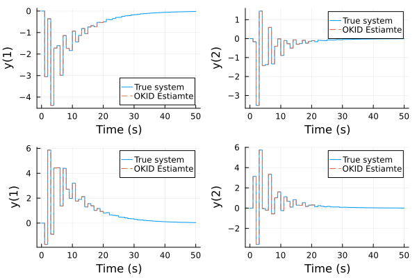

See the example notebooks for more details.

Estimate model from impulse-response data

The era ("Eigenvalue realization algorithm") and okid ("Observer Kalman identification") algorithms are often used together, where the latter estimates the Markov parameters (impulse response) and the former takes those and estimates a statespace model. If you have the Markov parameters already, you can call era directly to estimate a model from an impulse response.