Identification of nonlinear models

This package supports three forms of nonlinear system identification.

• Parameter estimation in a known model structure (linear or nonlinear) $x⁺ = f(x, u, p)$ where p is a vector of parameters to be estimated.
• Estimation of Hammerstein-Wiener models, i.e., linear systems with static nonlinear functions on the input and/or output.
• Estimation of Linear Parameter-Varying (LPV) state-space models, i.e., systems whose $A,B,C,D$ matrices depend on a measured scheduling variable $\lambda(t)$. This captures operating-point–dependent behavior of a nonlinear plant by interpolating between locally linear models.

Parameter estimation in a known model structure

Parameter estimation in differential equations can be performed by forming a one-step ahead predictor of the output, and minimizing the prediction error. This procedure is packaged in the function ControlSystemIdentification.nonlinear_pem which is available as a package extension, available if the user manually installs and loads LeastSquaresOptim.jl.

The procedure to use this function is as follows

1. The dynamics is specified on the form $x_{k+1} = f(x_k, u_k, p, t)$ or $ẋ = f(x, u, p, t)$ where $x$ is the state, $u$ the input, p is a vector of parameters to be estimated and $t$ is time.
2. If the dynamics is in continuous time (a differential equation or differential-algebraic equation), use the package SeeToDee.jl to discretize it. If the dynamics is already in discrete time, skip this step.
3. Define the measurement function $y = h(x, u, p, t)$ that maps the state and input to the measured output.
4. Specify covariance properties of the dynamics noise and measurement noise, similar to how one would do when building a Kalman filter for a linear system.
5. Perform the estimation using ControlSystemIdentification.nonlinear_pem.

Internally, ControlSystemIdentification.nonlinear_pem constructs an Unscented Kalman filter (UKF) from the package LowLevelParticleFilters.jl in order to perform state estimation along the provided data trajectory. An optimization problem is then solved in order to find the parameters (and optionally initial condition) that minimizes the prediction errors. This procedure is somewhat different from simply finding the parameters that make a pure simulation of the system match the data, notably, the prediction-error approach can usually handle very poor initial guesses, unstable systems and even chaotic systems. To learn more about the prediction-error method, see the tutorial Properties of the Prediction-Error Method.

nonlinear_pem(
    d::IdData,
    discrete_dynamics,
    measurement,
    p0,
    x0,
    R1,
    R2,
    nu;
    optimizer = LevenbergMarquardt(),
    λ = 1.0,
    optimize_x0 = true,
    kwargs...,
)

Example: Quad tank

This example considers a quadruple tank, where two upper tanks feed liquid into two lower tanks, depicted in the schematics below. The quad-tank process is a well-studied example in many multivariable control courses, this particular instance of the process is borrowed from the Lund University introductory course on automatic control.

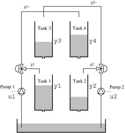
The process has a cross coupling between the tanks, governed by a parameters $\gamma_i$: The flows from the pumps are divided according to the two parameters $γ_1 , γ_2 ∈ [0, 1]$. The flow to tank 1 is $γ_1 k_1u_1$ and the flow to tank 4 is $(1 - γ_1 )k_1u_1$. Tanks 2 and 3 behave symmetrically.

The dynamics are given by

\[\begin{aligned} \dot{h}_1 &= \dfrac{-a_1}{A_1} \sqrt{2g h_1} + \dfrac{a_3}{A_1} \sqrt{2g h_3} + \dfrac{γ_1 k_1}{A_1} u_1 \\ \dot{h}_2 &= \dfrac{-a_2}{A_2} \sqrt{2g h_2} + \dfrac{a_4}{A_2} \sqrt{2g h_4} + \dfrac{γ_2 k_2}{A_2} u_2 \\ \dot{h}_3 &= \dfrac{-a_3}{A_3} \sqrt{2g h_3} + \dfrac{(1-γ_2) k_2}{A_3} u_2 \\ \dot{h}_4 &= \dfrac{-a_4}{A_4} \sqrt{2g h_4} + \dfrac{(1-γ_1) k_1}{A_4} u_1 \end{aligned}\]

where $h_i$ are the tank levels and $a_i, A_i$ are the cross-sectional areas of outlets and tanks respectively.

We start by defining the dynamics in continuous time, and discretize them using the integrator SeeToDee.Rk4 with a sample time of $T_s = 1$s.

using StaticArrays, SeeToDee

function quadtank(h, u, p, t)
    k1, k2, g = p[1], p[2], 9.81
    A1 = A3 = A2 = A4 = p[3]
    a1 = a3 = a2 = a4 = 0.03
    γ1 = γ2 = p[4]

    ssqrt(x) = √(max(x, zero(x)) + 1e-3) # For numerical robustness at x = 0

    SA[
        -a1/A1 * ssqrt(2g*h[1]) + a3/A1*ssqrt(2g*h[3]) +     γ1*k1/A1 * u[1]
        -a2/A2 * ssqrt(2g*h[2]) + a4/A2*ssqrt(2g*h[4]) +     γ2*k2/A2 * u[2]
        -a3/A3*ssqrt(2g*h[3])                          + (1-γ2)*k2/A3 * u[2]
        -a4/A4*ssqrt(2g*h[4])                          + (1-γ1)*k1/A4 * u[1]
    ]
end
measurement(x,u,p,t) = SA[x[1], x[2]]

Ts = 1.0
discrete_dynamics = SeeToDee.ForwardEuler(quadtank, Ts) # Use Heun, Rk3 or Rk4 if dynamics is more complex or sample rate is lower, ForwardEuler is fastest and higher-order methods do not provide any noticeable improvement in this particular case

(::SeeToDee.ForwardEuler{typeof(Main.quadtank), Float64}) (generic function with 1 method)

The output from this system is the water level in the first two tanks, i.e., $y = [x_1, x_2]$.

We also specify the number of state variables, outputs and inputs as well as a vector of "true" parameters, the ones we will try to estimate.

nx = 4
ny = 2
nu = 2
p_true = [1.6, 1.6, 4.9, 0.2]

4-element Vector{Float64}:
 1.6
 1.6
 4.9
 0.2

We then simulate some data from the system to use for identification:

using ControlSystemIdentification, ControlSystemsBase
using ControlSystemsBase.DemoSystems: resonant
using LowLevelParticleFilters
using LeastSquaresOptim
using Random, Plots, LinearAlgebra

# Generate some data from the system
Random.seed!(1)
Tperiod = 200
t = 0:Ts:1000
u1 = vcat.(0.25 .* sign.(sin.(2pi/Tperiod .* (t ./ 40).^2)) .+ 0.25)
u2 = vcat.(0.25 .* sign.(sin.(2pi/Tperiod .* (t ./ 40).^2 .+ pi/2)) .+ 0.25)
u  = vcat.(u1,u2)
u = [u; 0 .* u[1:100]]
x0 = [2.5, 1.5, 3.2, 2.8]
x = LowLevelParticleFilters.rollout(discrete_dynamics, x0, u, p_true)[1:end-1]
y = measurement.(x, u, 0, 0)
y = [y .+ 0.5randn(ny) for y in y] # Add some measurement noise
Y = reduce(hcat, y) # Go from vector of vectors to a matrix
U = reduce(hcat, u) # Go from vector of vectors to a matrix
plot(
    plot(reduce(hcat, x)', title="States", lab=["h1" "h2" "h3" "h4"]),
    plot(U', title="Inputs", lab=["u1" "u2"]),
    plot(Y', title="Outputs", lab=["y1" "y2"]),
)

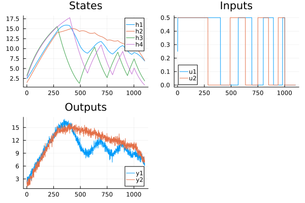
We package the experimental data into an iddata object as usual. Finally, we specify the covariance matrices for the dynamics noise and measurement noise as well as a guess for the initial condition. Since we can measure the level in the first two tanks, we use the true initial condition for those tanks, but we pretend that we are quite off when guessing the initial condition for the last two tanks.

Choosing the covariance matrices can be non-trivial, see the blog post How to tune a Kalman filter for some background. Here, we pick some value for $R_1$ that seems reasonable, and pick a deliberately large value for $R_2$. Choosing a large covariance of the measurement noise will lead to the state estimator trusting the measurements less, which in turns leads to a smaller feedback correction. This will make the algorithm favor a model that is good at simulation, rather than focusing exclusively on one-step prediction.

Finally, we call the function ControlSystemIdentification.nonlinear_pem to perform the estimation.

d = iddata(Y, U, Ts)
x0_guess = [2.5, 1.5, 1, 2] # Guess for the initial condition
p_guess = [1.4, 1.4, 5.1, 0.25] # Initial guess for the parameters

R1 = Diagonal([0.1, 0.1, 0.1, 0.1])
R2 = 100*Diagonal(0.5^2 * ones(ny))

model = ControlSystemIdentification.nonlinear_pem(d, discrete_dynamics, measurement, p_guess, x0_guess, R1, R2, nu)

NonlinearPredictionErrorModel
  p: [1.612854207115947, 1.599892556793933, 4.886859888419822, 0.2043195427487075]
  x0: [2.5596539594226195, 1.6758856247603915, 2.886780751913276, 2.106216431643522]
  Ts: 1.0
  ny = 2, nu = 2, nx = 4

We can then test how the model performs on the data, and compare with the model corresponding to our initial guess

simplot(model, d, layout=2)

x_guess = LowLevelParticleFilters.rollout(discrete_dynamics, x0_guess, u, p_guess)[1:end-1]
y_guess = measurement.(x_guess, u, 0, 0)
plot!(reduce(hcat, y_guess)', lab="Initial guess")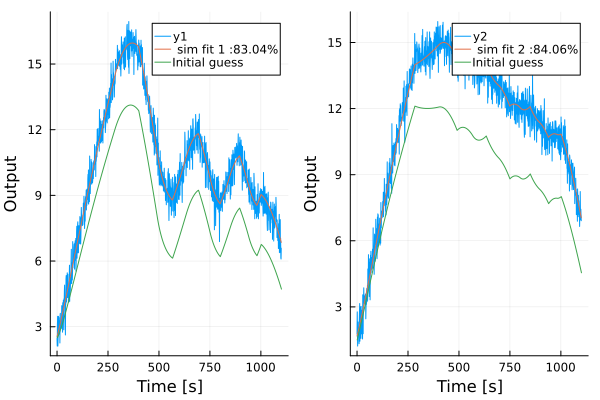

We can also perform a residual analysis to see if the model is able to capture the dynamics of the system

residualplot(model, d)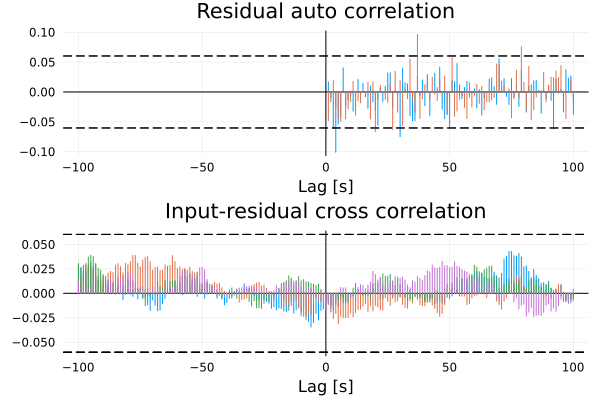

since we are using simulated data here, the residuals are white and there's nothing to worry about. In practice, one should always inspect the residuals to see if there are any systematic errors in the model.

Internally, the returned model object contains the estimated parameters, let's see if they are any good

[p_true p_guess model.p]

4×3 Matrix{Float64}:
 1.6  1.4   1.61285
 1.6  1.4   1.59989
 4.9  5.1   4.88686
 0.2  0.25  0.20432

hopefully, the estimated parameters are close to the true ones.

To customize the implementation of the nonlinear prediction-error method, see a lower-level interface being used in the tutorial in the documentation of LowLevelParticleFilters.jl which also provides the UKF.

Covariance of the estimated parameters

The object representing the estimated model contains a field Λ which is a function that returns an estimate of the precision matrix (inverse covariance matrix). Several caveats apply to this estimate, use with care. Example usage:

Σ = inv(model.Λ())
scatter(model.p, yerror=2sqrt.(diag(Σ[1:4, 1:4])), lab="Estimate")
scatter!(p_true, lab="True")
scatter!(p_guess, lab="Initial guess")

Hammerstein-Wiener estimation

This package provides elementary identification of nonlinear systems on Hammerstein-Wiener form, i.e., systems with a static input nonlinearity and a static output nonlinearity with a linear system in-between, where the nonlinearities are known. The only aspect of the nonlinearities that are optionally estimated are parameters. To formalize this, the estimation method newpem allows for estimation of a model of the form

\[\begin{aligned} x^+ &= Ax + B u_{nl} \\ y &= Cx + D u_{nl} \\ u_{nl} &= g_i(u, p) \\ y_{nl} &= g_o(y, p) \end{aligned}\]

   ┌─────┐   ┌─────┐   ┌─────┐
 u │     │uₙₗ│     │ y │     │ yₙₗ
──►│  gᵢ ├──►│  P  ├──►│  gₒ ├─►
   │     │   │     │   │     │
   └─────┘   └─────┘   └─────┘

where g_i and g_o are static, nonlinear functions that may depend on some parameter vector $p$ which is optimized together with the matrices $A,B,C,D$. The procedure to estimate such a model is detailed in the docstring for newpem.

The result of this estimation is the linear system without the nonlinearities applied, those must be handled manually by the user.

The default optimizer BFGS may struggle with problems including nonlinearities. If you do not get good results, try a different optimizer, e.g., optimizer = Optim.NelderMead().

Example with simulated data:

The example below identifies a model of a resonant system where the sign of the output is unknown, i.e., the output nonlinearity is given by $y_{nl} = |y|$. To make the example a bit more realistic, we also simulate colored measurement and input noise, yn and un. For an example with real data, see Hammerstein-Wiener estimation of nonlinear belt-drive system.

using ControlSystemIdentification, ControlSystemsBase
using ControlSystemsBase.DemoSystems: resonant
using Random, Plots

# Generate some data from the system
Random.seed!(1)
T = 200
sys = c2d(resonant(ω0 = 0.1) * tf(1, [0.1, 1]), 1)# generate_system(nx, nu, ny)
nx = sys.nx
nu = 1
ny = 1
x0 = zeros(nx)
sim(sys, u, x0 = x0) = lsim(sys, u, 1:T, x0 = x0)[1]
sysn = c2d(resonant(ω0 = 1) * tf(1, [0.1, 1]), 1)

σu = 1e-2 # Input noise standard deviation
σy = 1e-3 # Output noise standard deviation

u  = randn(nu, T)
un = u + sim(sysn, σu * randn(size(u)), 0 * x0)
y  = sim(sys, un, x0)
yn = y + sim(sysn, σy * randn(size(u)), 0 * x0)

# Nonlinear output transformation
ynn = abs.(yn)
d  = iddata(ynn, un, 1)
output_nonlinearity = (y, p) -> y .= abs.(y)

# Estimate 10 models with different random initialization and pick the best one
# If results are poor, try `optimizer = Optim.NelderMead()` instead
results = map(1:10) do _
    sysh, x0h, opt = newpem(d, nx; output_nonlinearity, show_trace=false, focus = :simulation)
    (; sysh, x0h, opt)
end;

(; sysh, x0h, opt) = argmin(r->r.opt.minimum, results) # Find the model with the smallest cost

yh = simulate(sysh, d, x0h)
output_nonlinearity(yh, nothing) # We need to manually apply the output nonlinearity to the prediction
plot(d.t, [abs.(y); u]', lab=["True nonlinear output" "Input"], seriestype = [:line :steps], layout=(2,1), xlabel="Time")
scatter!(d.t, ynn', lab="Measured nonlinear output", sp=1)
plot!(d.t, yh', lab="Simulation", sp=1, l=:dash)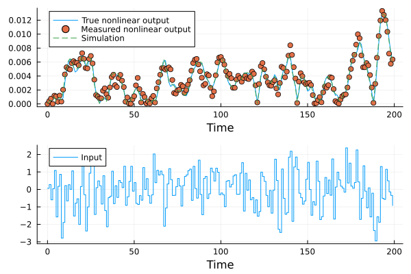

Linear Parameter-Varying (LPV) identification

lpv_pem fits a state-space model whose matrices depend on a measured scheduling variable $\lambda(t)$ through a user-supplied basis expansion, $A(\lambda) = \sum_k A_k\, \varphi_k(\lambda)$ and likewise for $B,C,D$. The returned LPVStateSpace is callable: sys(λ) returns a plain StateSpace frozen at that operating point.

sys, x0, res = lpv_pem( d,  λ,  nx; basis, ...)
sys, x0, res = lpv_pem(ds, λs, nx; basis, ...)

A(λ) = Σ_k A_k φ_k(λ),     ...,     D(λ) = Σ_k D_k φ_k(λ).

A0 = [0.9 0.1; 0 0.8]; A1 = [0.0 0.0; 0.05 0.0]
B0 = [0.1; 0.2;;];     B1 = [0.0; 0.05;;]
C  = [1.0 0.0]; Ts = 0.05
T  = 2000
λ  = sin.(0.01 .* (1:T))
u  = randn(1, T)
A(λ) = A0 .+ λ .* A1
B(λ) = B0 .+ λ .* B1

x = zeros(2); y = zeros(1, T)
for t in 1:T
    y[:, t] = C * x
    x = A(λ[t]) * x + B(λ[t]) * u[:, t]
end
y .+= 0.01 .* randn(size(y))
d = iddata(y, u, Ts)

basis = [_ -> 1.0, λ -> λ]
sys, x0h, res = lpv_pem(d, λ, 2; basis)

lpv_warmstart(d,  λ,  nx; basis, window = nothing, stride = nothing) -> ComponentArray
lpv_warmstart(ds, λs, nx; basis, window = nothing, stride = nothing) -> ComponentArray

See Linear Parameter-Varying (LPV) identification for a worked example.

Video tutorials

Relevant video tutorials are available here: